
6.7: Solving Equilibrium Problems
- Page ID
- 5716

\( \newcommand{\vecs}[1]{\overset { \scriptstyle \rightharpoonup} {\mathbf{#1}} } \)
\( \newcommand{\vecd}[1]{\overset{-\!-\!\rightharpoonup}{\vphantom{a}\smash {#1}}} \)
\( \newcommand{\id}{\mathrm{id}}\) \( \newcommand{\Span}{\mathrm{span}}\)
( \newcommand{\kernel}{\mathrm{null}\,}\) \( \newcommand{\range}{\mathrm{range}\,}\)
\( \newcommand{\RealPart}{\mathrm{Re}}\) \( \newcommand{\ImaginaryPart}{\mathrm{Im}}\)
\( \newcommand{\Argument}{\mathrm{Arg}}\) \( \newcommand{\norm}[1]{\| #1 \|}\)
\( \newcommand{\inner}[2]{\langle #1, #2 \rangle}\)
\( \newcommand{\Span}{\mathrm{span}}\)
\( \newcommand{\id}{\mathrm{id}}\)
\( \newcommand{\Span}{\mathrm{span}}\)
\( \newcommand{\kernel}{\mathrm{null}\,}\)
\( \newcommand{\range}{\mathrm{range}\,}\)
\( \newcommand{\RealPart}{\mathrm{Re}}\)
\( \newcommand{\ImaginaryPart}{\mathrm{Im}}\)
\( \newcommand{\Argument}{\mathrm{Arg}}\)
\( \newcommand{\norm}[1]{\| #1 \|}\)
\( \newcommand{\inner}[2]{\langle #1, #2 \rangle}\)
\( \newcommand{\Span}{\mathrm{span}}\) \( \newcommand{\AA}{\unicode[.8,0]{x212B}}\)
\( \newcommand{\vectorA}[1]{\vec{#1}} % arrow\)
\( \newcommand{\vectorAt}[1]{\vec{\text{#1}}} % arrow\)
\( \newcommand{\vectorB}[1]{\overset { \scriptstyle \rightharpoonup} {\mathbf{#1}} } \)
\( \newcommand{\vectorC}[1]{\textbf{#1}} \)
\( \newcommand{\vectorD}[1]{\overrightarrow{#1}} \)
\( \newcommand{\vectorDt}[1]{\overrightarrow{\text{#1}}} \)
\( \newcommand{\vectE}[1]{\overset{-\!-\!\rightharpoonup}{\vphantom{a}\smash{\mathbf {#1}}}} \)
\( \newcommand{\vecs}[1]{\overset { \scriptstyle \rightharpoonup} {\mathbf{#1}} } \)
\( \newcommand{\vecd}[1]{\overset{-\!-\!\rightharpoonup}{\vphantom{a}\smash {#1}}} \)
\(\newcommand{\avec}{\mathbf a}\) \(\newcommand{\bvec}{\mathbf b}\) \(\newcommand{\cvec}{\mathbf c}\) \(\newcommand{\dvec}{\mathbf d}\) \(\newcommand{\dtil}{\widetilde{\mathbf d}}\) \(\newcommand{\evec}{\mathbf e}\) \(\newcommand{\fvec}{\mathbf f}\) \(\newcommand{\nvec}{\mathbf n}\) \(\newcommand{\pvec}{\mathbf p}\) \(\newcommand{\qvec}{\mathbf q}\) \(\newcommand{\svec}{\mathbf s}\) \(\newcommand{\tvec}{\mathbf t}\) \(\newcommand{\uvec}{\mathbf u}\) \(\newcommand{\vvec}{\mathbf v}\) \(\newcommand{\wvec}{\mathbf w}\) \(\newcommand{\xvec}{\mathbf x}\) \(\newcommand{\yvec}{\mathbf y}\) \(\newcommand{\zvec}{\mathbf z}\) \(\newcommand{\rvec}{\mathbf r}\) \(\newcommand{\mvec}{\mathbf m}\) \(\newcommand{\zerovec}{\mathbf 0}\) \(\newcommand{\onevec}{\mathbf 1}\) \(\newcommand{\real}{\mathbb R}\) \(\newcommand{\twovec}[2]{\left[\begin{array}{r}#1 \\ #2 \end{array}\right]}\) \(\newcommand{\ctwovec}[2]{\left[\begin{array}{c}#1 \\ #2 \end{array}\right]}\) \(\newcommand{\threevec}[3]{\left[\begin{array}{r}#1 \\ #2 \\ #3 \end{array}\right]}\) \(\newcommand{\cthreevec}[3]{\left[\begin{array}{c}#1 \\ #2 \\ #3 \end{array}\right]}\) \(\newcommand{\fourvec}[4]{\left[\begin{array}{r}#1 \\ #2 \\ #3 \\ #4 \end{array}\right]}\) \(\newcommand{\cfourvec}[4]{\left[\begin{array}{c}#1 \\ #2 \\ #3 \\ #4 \end{array}\right]}\) \(\newcommand{\fivevec}[5]{\left[\begin{array}{r}#1 \\ #2 \\ #3 \\ #4 \\ #5 \\ \end{array}\right]}\) \(\newcommand{\cfivevec}[5]{\left[\begin{array}{c}#1 \\ #2 \\ #3 \\ #4 \\ #5 \\ \end{array}\right]}\) \(\newcommand{\mattwo}[4]{\left[\begin{array}{rr}#1 \amp #2 \\ #3 \amp #4 \\ \end{array}\right]}\) \(\newcommand{\laspan}[1]{\text{Span}\{#1\}}\) \(\newcommand{\bcal}{\cal B}\) \(\newcommand{\ccal}{\cal C}\) \(\newcommand{\scal}{\cal S}\) \(\newcommand{\wcal}{\cal W}\) \(\newcommand{\ecal}{\cal E}\) \(\newcommand{\coords}[2]{\left\{#1\right\}_{#2}}\) \(\newcommand{\gray}[1]{\color{gray}{#1}}\) \(\newcommand{\lgray}[1]{\color{lightgray}{#1}}\) \(\newcommand{\rank}{\operatorname{rank}}\) \(\newcommand{\row}{\text{Row}}\) \(\newcommand{\col}{\text{Col}}\) \(\renewcommand{\row}{\text{Row}}\) \(\newcommand{\nul}{\text{Nul}}\) \(\newcommand{\var}{\text{Var}}\) \(\newcommand{\corr}{\text{corr}}\) \(\newcommand{\len}[1]{\left|#1\right|}\) \(\newcommand{\bbar}{\overline{\bvec}}\) \(\newcommand{\bhat}{\widehat{\bvec}}\) \(\newcommand{\bperp}{\bvec^\perp}\) \(\newcommand{\xhat}{\widehat{\xvec}}\) \(\newcommand{\vhat}{\widehat{\vvec}}\) \(\newcommand{\uhat}{\widehat{\uvec}}\) \(\newcommand{\what}{\widehat{\wvec}}\) \(\newcommand{\Sighat}{\widehat{\Sigma}}\) \(\newcommand{\lt}{<}\) \(\newcommand{\gt}{>}\) \(\newcommand{\amp}{&}\) \(\definecolor{fillinmathshade}{gray}{0.9}\)Ladder diagrams are a useful tool for evaluating chemical reactivity, usually providing a reasonable approximation of a chemical system’s composition at equilibrium. If we need a more exact quantitative description of the equilibrium condition, then a ladder diagram is insufficient. In this case we need to find an algebraic solution. In this section we will learn how to set-up and solve equilibrium problems. We will start with a simple problem and work toward more complex problems.
6.7.1 A Simple Problem—Solubility of Pb(IO3)2
If we place an insoluble compound such as Pb(IO3)2 in deionized water, the solid dissolves until the concentrations of Pb2+ and IO3– satisfy the solubility product for Pb(IO3)2. At equilibrium the solution is saturated with Pb(IO3)2, which simply means that no more solid can dissolve. How do we determine the equilibrium concentrations of Pb2+ and IO3–, and what is the molar solubility of Pb(IO3)2 in this saturated solution?
When we first add solid Pb(IO3)2 to water, the concentrations of Pb2+ and IO3– are zero and the reaction quotient, Q, is
\[Q=\mathrm{[Pb^{2+}][ \sideset{}{_{3}^{-}}{IO} ]^2}=0\]
As the solid dissolves, the concentrations of these ions increase, but Q remains smaller than Ksp. We reach equilibrium and “satisfy the solubility product” when
\[Q=K_\mathrm{sp}\]
We begin by writing the equilibrium reaction and the solubility product expression for Pb(IO3)2.
\[\mathrm{Pb(IO_3)_2}(s)\rightleftharpoons\mathrm{Pb^{2+}}(aq)+\mathrm{2 \sideset{}{_{3}^{-}}{IO} }(aq)\]
\[K_\mathrm{sp}=\mathrm{[Pb^{2+}][ \sideset{}{_{3}^{-}}{IO} ]^2}=2.5\times10^{-13}\tag{6.33}\]
As Pb(IO3)2 dissolves, two IO3– ions are produced for each ion of Pb2+. If we assume that the change in the molar concentration of Pb2+ at equilibrium is x, then the change in the molar concentration of IO3– is 2x. The following table helps us keep track of the initial concentrations, the change in concentrations, and the equilibrium concentrations of Pb2+ and IO3–.
| Concentrations | Pb(IO3)2 (s) | ⇋ | Pb2+ (aq) | + | 2IO3– (aq) | |
| Initial | solid | 0 | 0 | |||
|
Change |
solid |
+x |
+2x |
|||
| Equilibrium | solid | x | 2x | |||
Because a solid, such as Pb(IO3)2, does not appear in the solubility product expression, we do not need to keep track of its concentration. Remember, however, that the Ksp value applies only if there is some Pb(IO3)2 present at equilibrium.
Substituting the equilibrium concentrations into equation 6.33 and solving gives
\[(x)(2x)^2=4x^3=2.5\times10^{-13}\]
\[x=3.97\times10^{-5}\]
Substituting this value of x back into the equilibrium concentration expressions for Pb2+ and IO3– gives their concentrations as
\[\mathrm{[Pb^{2+}]}=x=4.0\times10^{-5}\textrm{ M}\]
\[\mathrm{[ \sideset{}{_{3}^{-}}{IO} ]}=2x=7.9\times10^{-5}\textrm{ M}\]
Because one mole of Pb(IO3)2 contains one mole of Pb2+, the molar solubility of Pb(IO3)2 is equal to the concentration of Pb2+, or 4.0 × 10⁻⁵ M.
We can express a compound’s solubility in two ways: molar solubility (mol/L) or mass solubility (g/L). Be sure to express your answer clearly.
Exercise 6.7
Calculate the molar solubility and the mass solubility for Hg2Cl2, given the following solubility reaction and Ksp value.
\[\mathrm{Hg_2Cl_2}(s)\rightleftharpoons\mathrm{Hg_2^{2+}}(aq)+\mathrm{2Cl^-}(aq)\hspace{9mm}K_\mathrm{sp}=1.2\times10^{-18}\]
Click here to review your answer to this exercise.
6.7.2 A More Complex Problem—The Common Ion Effect
Calculating the solubility of Pb(IO3)2 in deionized water is a straightforward problem since the solid’s dissolution is the only source of Pb2+ and IO3–. But what if we add Pb(IO3)2 to a solution of 0.10 M Pb(NO3)2, which provides a second source of Pb2+? Before we set-up and solve this problem algebraically, think about the system’s chemistry and decide whether the solubility of Pb(IO3)2 will increase, decrease or remain the same.
Beginning a problem by thinking about the likely answer is a good habit to develop. Knowing what answers are reasonable will help you spot errors in your calculations and give you more confidence that your solution to a problem is correct.
Because the solution already contains a source of Pb2+, we can use Le Châtelier’s principle to predict that the solubility of Pb(IO3)2 is smaller than that in our previous problem.
We begin by setting up a table to help us keep track of the concentrations of Pb2+ and IO3– as this system moves toward and reaches equilibrium.
| Concentrations | Pb(IO3)2 (s) | ⇋ | Pb2+ (aq) | + | 2IO3– (aq) | |
|
Initial Change |
solid solid |
0.10 +x |
0 +2x |
|||
| Equilibrium | solid | 0.10 + x | 2x | |||
Substituting the equilibrium concentrations into equation 6.33
\[(0.10+x)(2x)^2=2.5\times10^{-13}\]
and multiplying out the terms on the equation’s left side leaves us with
\[4x^3+0.40x^2=2.5\times10^{-13}\tag{6.34}\]
This is a more difficult equation to solve than that for the solubility of Pb(IO3)2 in deionized water, and its solution is not immediately obvious. We can find a rigorous solution to equation 6.34 using available computer software packages and spreadsheets, some of which are described in Section 6.J.
Note
There are several approaches to solving cubic equations, but none are computationally easy.
How might we solve equation 6.34 if we do not have access to a computer? One approach is to use our understanding of chemistry to simplify the problem. From Le Châtelier’s principle we know that a large initial concentration of Pb2+ significantly decreases the solubility of Pb(IO3)2. One reasonable assumption is that the equilibrium concentration of Pb2+ is very close to its initial concentration. If this assumption is correct, then the following approximation is reasonable
\[\mathrm{[Pb^{2+}]}=0.10+x\approx0.10\textrm{ M}\]
Substituting our approximation into equation 6.33 and solving for x gives
\[(0.1)(2x)^2=2.5\times10^{-13}\]
\[0.4x^2=2.5\times10^{-13}\]
\[x=7.91\times10^{-7}\]
Before accepting this answer, we must verify that our approximation is reasonable. The difference between the calculated concentration of Pb2+, 0.10 + x M, and our assumption that it is 0.10 M is 7.9 × 10⁻⁷, or 7.9 × 10⁻⁴% of the assumed concentration. This is a negligible error.
Note
\[\begin{align}
\mathrm{\%error}&=\dfrac{(0.10+x)-0.10}{0.10}\times100\\
&=\dfrac{7.91\times10^{-7}}{0.10}\times100\\
&=7.91\times10^{-4}\%
\end{align}\]
Accepting the result of our calculation, we find that the equilibrium concentrations of Pb2+ and IO3– are
\[\mathrm{[Pb^{2+}]}=0.10+x\approx\textrm{0.10 M}\]
\[\mathrm{[ \sideset{}{_{3}^{-}}{IO} ]}=2x=1.6\times10^{-6}\textrm{ M}\]
The molar solubility of Pb(IO3)2 is equal to the additional concentration of Pb2+ in solution, or 7.9 × 10⁻⁴ mol/L. As expected, Pb(IO3)2 is less soluble in the presence of a solution that already contains one of its ions. This is known as the common ion effect.
As outlined in the following example, if an approximation leads to an unacceptably large error we can extend the process of making and evaluating approximations.
Example 6.10
Calculate the solubility of Pb(IO3)2 in 1.0 × 10⁻⁴ M Pb(NO3)2.
Solution
Letting x equal the change in the concentration of Pb2+, the equilibrium concentrations of Pb2+ and IO3– are
\[\mathrm{[Pb^{2+}]}=1.0\times10^{-4}+x\hspace{8mm}\mathrm{[ \sideset{}{_{3}^{-}}{IO} ]}=2x\]
Substituting these concentrations into equation 6.33 leaves us with
\[(1.0\times10^{-4}+x)(2x)^2=2.5\times10^{-13}\]
To solve this equation for x, we make the following assumption
\[\mathrm{[Pb^{2+}]}=1.0\times10^{-4}+x\approx1.0\times10^{-4}\textrm{ M}\]
obtaining a value for x of 2.50×10⁻⁴. Substituting back, gives the calculated concentration of Pb2+ at equilibrium as
\[\mathrm{[Pb^{2+}]=1.0\times10^{-4}+2.50\times10^{-5}=1.25\times10^{-4}\;M}\]
a value that differs by 25% from our assumption that the equilibriumconcentration is 1.0×10⁻⁴ M. This error seems unreasonably large. Rather than shouting in frustration, we make a new assumption. Our first assumption—that the concentration of Pb2+ is 1.0×10⁻⁴ M—was too small. The calculated concentration of 1.25×10⁻⁴ M, therefore, is probably a bit too large. For our second approximation, let’s assume that
\[\mathrm{[Pb^{2+}]}=1.0\times10^{-4}+x\approx1.25\times10^{-4}\]
Substituting into equation 6.33 and solving for x gives its value as 2.24× 10⁻⁵. The resulting concentration of Pb2+ is
\[\mathrm{[Pb^{2+}]=1.0\times10^{-4}+2.24\times10^{-5}=1.22\times10^{-4}\;M}\]
which differs from our assumption of 1.25× 10–4 M by 2.4%. Because the original concentration of Pb2+ is given to two significant figure, this is a more reasonable error. Our final solution, to two significant figures, is
\[\mathrm{[Pb^{2+}]=1.2\times10^{-4}\;M\hspace{7mm}[ \sideset{}{_{3}^{-}}{IO} ]=4.5\times10^{-5}\;M}\]
and the molar solubility of Pb(IO3)2 is 2.2× 10⁻⁵ mol/L. This iterative approach to solving an equation is known as the method of successive approximations.
Practice Exercise 6.8
Calculate the molar solubility for Hg2Cl2 in 0.10 M NaCl and compare your answer to its molar solubility in deionized water (see Practice Exercise 6.7).Click here to review your answer to this exercise.
6.7.3 A Systematic Approach to Solving Equilibrium Problems
Calculating the solubility of Pb(IO3)2 in a solution of Pb(NO3)2 is more complicated than calculating its solubility in deionized water. The calculation, however, is still relatively easy to organize, and the simplifying assumption fairly obvious. This problem is reasonably straightforward because it involves only one equilibrium reaction and one equilibrium constant.
Determining the equilibrium composition of a system with multiple equilibrium reactions is more complicated. In this section we introduce a systematic approach to setting‑up and solving equilibrium problems. As shown in Table 6.1, this approach involves four steps.
| Step 1: Write all relevant equilibrium reactions and equilibrium constant expressions. |
| Step 2: Count the unique species appearing in the equilibrium constant expressions; these are your unknowns. You have enough information to solve the problem if the number of unknowns equals the number of equilibrium constant expressions. If not, add a mass balance equation and/or a charge balance equation. Continue adding equations until the number of equations equals the number of unknowns. |
| Step 3: Combine your equations and solve for one unknown. Whenever possible, simplify the algebra by making appropriate assumptions. If you make an assumption, set a limit for its error. This decision influences your evaluation of the assumption. |
| Step 4: Check your assumptions. If any assumption proves invalid, return to the previous step and continue solving. The problem is complete when you have an answer that does not violate any of your assumptions. |
In addition to equilibrium constant expressions, two other equations are important to the systematic approach for solving equilibrium problems. The first of these is a mass balance equation, which is simply a statement that matter is conserved during a chemical reaction. In a solution of a acetic acid, for example, the combined concentrations of the conjugate weak acid, CH3COOH, and the conjugate weak base, CH3COO–, must equal acetic acid’s initial concentration, CCH3COOH.
\[C_\mathrm{CH_3COOH}=\mathrm{[CH_3COOH]+[CH_3COO^-]}\]
Note
You may recall from Chapter 2 that this is the difference between a formal concentration and a molar concentration. The variable C represents a formal concentration.
The second equation is a charge balance equation, which requires that total charge from the cations equal the total charge from the anions. Mathematically, the charge balance equation is
\[\sum_{i}|(z^+)_i|[\textrm C^{z+}]_i=\sum_{j}|(z^-)_j|[\textrm A^{z-}]_j\]
where [Cz+]i and [Az−]j are, respectively, the concentrations of the ith cation and the jth anion, and |(z+)i| and |(z−)j| are the absolute values of theith cation’s charge and the jth anion’s charge. Every ion in solution, even if it does not appear in an equilibrium reaction, must appear in the charge balance equation. For example, the charge balance equation for an aqueous solution of Ca(NO3)2 is
\[\mathrm{2\times[Ca^{2+}]+[H_3O^+]=[OH^-]+[ \sideset{}{_{3}^{-}}{NO}]}\]
Note that we multiply the concentration of Ca2+ by two, and that we include the concentrations of H3O+ and OH–.
Note
We use absolute values because we are balancing the concentration of charge and concentrations cannot be negative.
There are situations where it is impossible to write a charge balance equation because we do not have enough information about the solution’s composition. For example, suppose we fix a solution’s pH using a buffer. If the buffer’s composition is not specified, then a charge balance equation can not be written.
Example 6.11
Write mass balance equations and a charge balance equation for a 0.10 M solution of NaHCO3.
Solution
It is easier to keep track of the species in solution if we write down the reactions controlling the solution’s composition. These reactions are the dissolution of a soluble salt
\[\mathrm{NaHCO_3}(s)\rightarrow\mathrm{Na^+}(aq)+\mathrm{ \sideset{}{_{3}^{-}}{HCO} }(aq)\]
and the acid–base dissociation reactions of HCO3– and H2O
\[\mathrm{ \sideset{}{_{3}^{-}}{HCO} }(aq)+\mathrm{H_2O}(l)\rightleftharpoons\mathrm{H_3O^+}(aq)+\mathrm{CO_3^{2-}}(aq)\]
\[\mathrm{ \sideset{}{_{3}^{-}}{HCO} }(aq)+\mathrm{H_2O}(l)\rightleftharpoons\mathrm{OH^-}(aq)+\mathrm{H_2CO_3}(aq)\]
\[\mathrm{2H_2O}(l)\rightleftharpoons\mathrm{H_3O^+}(aq)+\mathrm{OH^-}(aq)\]
The mass balance equations are
\[\mathrm{0.10\;M=[H_2CO_3]+[ \sideset{}{_{3}^{-}}{HCO} ]+[CO_3^{2-}]}\]
\[\mathrm{0.10\;M=[Na^+]}\]
and the charge balance equation is
\[\mathrm{[Na^+]+[H_3O^+]=[OH^-]+[ \sideset{}{_{3}^{-}}{HCO} ]+2\times[CO_3^{2-}]}\]
Practice Exercise 6.9
Write appropriate mass balance and charge balance equations for a solution containing 0.10 M KH2PO4 and 0.050 M Na2HPO4.
Click here to review your answer to this exercise.
6.7.4 pH of a Monoprotic Weak Acid
To illustrate the systematic approach to solving equilibrium problems, let’s calculate the pH of 1.0 M HF. (Step 1: Write all relevant equilibrium reactions and equilibrium constant expressions.) Two equilibrium reactions affect the pH. The first, and most obvious, is the acid dissociation reaction for HF
\[\mathrm{HF}(aq)+\mathrm{H_2O}(l)\rightleftharpoons\mathrm{H_3O^+}(aq)+\mathrm{F^-}(aq)\]
for which the equilibrium constant expression is
\[K_\textrm a=\mathrm{\dfrac{[H_3O^+][F^-]}{[HF]}}=6.8\times10^{-4}\tag{6.35}\]
The second equilibrium reaction is the dissociation of water, which is an obvious yet easily neglected reaction
\[\mathrm{2H_2O}(l)\rightleftharpoons\mathrm{H_3O^+}(aq)+\mathrm{OH^-}(aq)\]
\[K_\textrm w=\mathrm{[H_3O^+][OH^-]}=1.00\times10^{-14}\tag{6.36}\]
Note
Step 2: Count the unique species appearing in the equilibrium constant expressions; these are your unknowns. You have enough information to solve the problem if the number of unknowns equals the number of equilibrium constant expressions. If not, add a mass balance equation and/or a charge balance equation. Continue adding equations until the number of equations equals the number of unknowns.
Counting unknowns, we find four: [HF], [F−], [H3O+], and [OH−]. To solve this problem we need two additional equations. These equations are a mass balance equation on hydrofluoric acid
\[C_\textrm{HF}=\mathrm{[HF]+[F^-]}\tag{6.37}\]
and a charge balance equation
\[\mathrm{[H_3O^+]=[OH^-]+[F^-]}\tag{6.38}\]
With four equations and four unknowns, we are ready to solve the problem. Before doing so, let’s simplify the algebra by making two assumptions.
Note
Step 3: Combine your equations and solve for one unknown. Whenever possible, simplify the algebra by making appropriate assumptions. If you make an assumption, set a limit for its error. This decision influences your evaluation the assumption.
Assumption One. Because HF is a weak acid, the solution must be acidic. For an acidic solution it is reasonable to assume that
\[\mathrm{[H_3O^+]>>[OH^-]}\]
which simplifies the charge balance equation to
\[\mathrm{[H_3O^+]=[F^-]}\tag{6.39}\]
Assumption Two. Because HF is a weak acid, very little dissociation occurs. Most of the HF remains in its conjugate weak acid form and it is reasonable to assume that
\[\mathrm{[HF]>>[F^-]}\]
which simplifies the mass balance equation to
\[C_\mathrm{HF}=\mathrm{[HF]}\tag{6.40}\]
For this exercise let’s accept an assumption if it introduces an error of less than ±5%.
Substituting equation 6.39 and equation 6.40 into equation 6.35, and solving for the concentration of H3O+ gives us
\[\mathrm{\mathit K_a=\dfrac{[H_3O^+][H_3O^+]}{\mathit C_{HF}}=\dfrac{[H_3O^+]^2}{\mathit C_{HF}}=6.8\times10^{-4}}\]
\[\mathrm{[H_3O^+]}=\sqrt{K_\mathrm aC_\mathrm {HF}}=\sqrt{(6.8\times10^{-4})(1.0)}=2.6\times10^{-2}\]
Note
Step 4: Check your assumptions. If any assumption proves invalid, return to the previous step and continue solving. The problem is complete when you have an answer that does not violate any of your assumptions.
Before accepting this answer, we must verify our assumptions. The first assumption is that [OH−] is significantly smaller than [H3O+]. Using equation 6.36, we find that
\[\mathrm{[OH^-]}=\dfrac{K_\mathrm w}{\mathrm{[H_3O^+]}}=\dfrac{1.00\times10^{-14}}{2.6\times10^{-2}}=3.8\times10^{-13}\]
Clearly this assumption is acceptable. The second assumption is that [F−] is significantly smaller than [HF]. From equation 6.39 we have
\[\mathrm{[F^-]=2.6\times10^{-2}\;M}\]
Because [F−] is 2.60% of CHF, this assumption is also acceptable. Given that [H3O+] is 2.6 × 10⁻² M, the pH of 1.0 M HF is 1.59.
How does the calculation change if we limit an assumption’s error to less than ±1%? In this case we can no longer assume that [HF] >> [F−] and we cannot simplify the mass balance equation. Solving the mass balance equation for [HF]
\[\mathrm{[HF]}=C_\textrm{HF}-[\mathrm F^-]=C_\textrm{HF}-\mathrm{[H_3O^+]}\]
and substituting into theKa expression along with equation 6.39 gives
\[K_\mathrm a=\dfrac{\mathrm{[H_3O^+]^2}}{C_\mathrm{HF}-\mathrm{[H_3O^+]}}\]
Rearranging this equation leaves us with a quadratic equation
\[\mathrm{[H_3O^+]^2}+K_\mathrm a\mathrm{[H_3O^+]}-K_\mathrm aC_\mathrm{HF}=0\]
which we solve using the quadratic formula
\[x=\dfrac{-b\pm\sqrt{b^2-4ac}}{2a}\]
where a, b, and c are the coefficients in the quadratic equation
\[ax^2+bx+c=0\]
Solving a quadratic equation gives two roots, only one of which has chemical significance. For our problem, the equation’s roots are
\[x=\dfrac{-6.8\times10^{-4}\pm\sqrt{(6.8\times10^{-4})^2-(4)(1)(6.8\times10^{-4})}}{(2)(1)}\]
\[x=\dfrac{-6.8\times10^{-4}\pm5.22\times10^{-2}}{2}\]
\[x=2.57\times10^{-2}\textrm{ or }-2.63\times10^{-2}\]
Only the positive root is chemically significant because the negative root gives a negative concentration for H3O+. Thus, [H3O+] is 2.6 × 10⁻² M and the pH is 1.59.
You can extend this approach to calculating the pH of a monoprotic weak base by replacing Ka with Kb, replacing CHF with the weak base’s concentration, and solving for [OH−] in place of [H3O+].
Practice Exercise 6.10
Calculate the pH of 0.050 M NH3. State any assumptions you make in solving the problem, limiting the error for any assumption to ±5%. The Kb value for NH3 is 1.75 × 10⁻⁵.
Click here to review your answer to this exercise.
6.7.5 pH of a Polyprotic Acid or Base
A more challenging problem is to find the pH of a solution containing a polyprotic weak acid or one of its conjugate species. As an example, consider the amino acid alanine, whose structure is shown in Figure 6.12. The ladder diagram in Figure 6.13 shows alanine’s three acid–base forms and their respective areas of predominance. For simplicity, we identify these species as H2L+, HL, and L–.
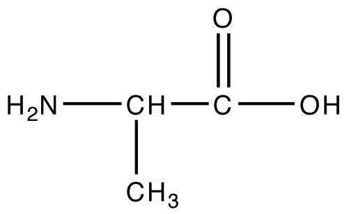
Figure 6.12 Structure of the amino acid alanine, which has pKa values of 2.348 and 9.867.
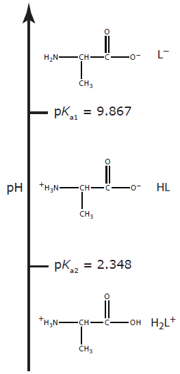
Figure 6.13 Ladder diagram for alanine.
pH of 0.10 M Alanine Hydrochloride (H2L+)
Alanine hydrochloride is a salt of the diprotic weak acid H2L+ and Cl–. Because H2L+ has two acid dissociation reactions, a complete systematic solution to this problem is more complicated than that for a monoprotic weak acid. The ladder diagram in Figure 6.13 helps us simplify the problem. Because the areas of predominance for H2L+ and L– are so far apart, we can assume that a solution of H2L+ is not likely to contain significant amounts of L–. As a result, we can treat H2L+ as though it is a monoprotic weak acid. Calculating the pH of 0.10 M alanine hydrochloride, which is 1.72, is left to the reader as an exercise.
pH of 0.10 M Sodium Alaninate (L–)
The alaninate ion is a diprotic weak base. Because L– has two base dissociation reactions, a complete systematic solution to this problem is more complicated than that for a monoprotic weak base. Once again, the ladder diagram in Figure 6.13 helps us simplify the problem. Because the areas of predominance for H2L+ and L– are so far apart, we can assume that a solution of L– is not likely to contain significant amounts of H2L+. As a result, we can treat L– as though it is a monoprotic weak base. Calculating the pH of 0.10 M sodium alaninate, which is 11.42, is left to the reader as an exercise.
pH of 0.1 M Alanine (HL)
Finding the pH of a solution of alanine is more complicated than our previous two examples because we cannot ignore the presence of both H2L+ and L–. To calculate the solution’s pH we must consider alanine’s acid dissociation reaction
\[\mathrm{HL}(aq)+\mathrm{H_2O}(l)\rightleftharpoons\mathrm{H_3O^+}(aq)+\mathrm{L^-}(aq)\]
and its base dissociation reaction
\[\mathrm{HL}(aq)+\mathrm{H_2O}(l)\rightleftharpoons\mathrm{OH^-}(aq)+\mathrm{H_2L^+}(aq)\]
As always, we must also consider the dissociation of water
\[\mathrm{2H_2O}(l)\rightleftharpoons\mathrm{H_3O^+}(aq)+\mathrm{OH^-}(aq)\]
This leaves us with five unknowns—[H2L+], [HL], [L−], [H3O+], and [OH−]—for which we need five equations. These equations are Ka2 and Kb2 for alanine
\[K_\mathrm{a2}=\mathrm{\dfrac{[H_3O^+][L^-]}{[HL]}}\]
\[K_\mathrm{b2}=\dfrac{K_\mathrm w}{K_\mathrm{a1}}=\mathrm{\dfrac{[OH^-][H_2L^+]}{[HL]}}\]
the Kw equation
\[K_\mathrm w=\mathrm{[H_3O^+][OH^-]}\]
a mass balance equation for alanine
\[C_\mathrm{HL}=\mathrm{[H_2L^+]+[HL]+[L^-]}\]
and a charge balance equation
\[\mathrm{[H_2L^+]+[H_3O^+]=[OH^-]+[L^-]}\]
Because HL is a weak acid and a weak base, it seems reasonable to assume that
\[\mathrm{[HL]>>[H_2L^+]+[L^-]}\]
which allows us to simplify the mass balance equation to
\[C_\mathrm{HL}=\mathrm{[HL]}\]
Next we solve Kb2 for [H2L+]
\[\mathrm{[H_2L^+]=\dfrac{\mathit K_w[HL]}{\mathit K_{a1}[OH^-]}=\dfrac{[H_3O^+][HL]}{\mathit K_{a1}}=\dfrac{\mathit C_{HL}[H_3O^+]}{\mathit K_{a1}}}\]
and Ka2 for [L−]
\[\mathrm{[L^-]=\dfrac{\mathit K_{a2}[HL]}{[H_3O^+]}=\dfrac{\mathit K_{a2}\mathit C_{HL}}{[H_3O^+]}}\]
Substituting these equations for [H2L+] and [L−], along with the equation for Kw, into the charge balance equation give us
\[\mathrm{\dfrac{\mathit C_{HL}[H_3O^+]}{\mathit K_{a1}}+[H_3O^+]=\dfrac{\mathit K_w}{[H_3O^+]}+\dfrac{\mathit K_{a2}\mathit C_{HL}}{[H_3O^+]}}\]
which we simplify to
\[\mathrm{[H_3O^+]\dfrac{\mathit C_{HL}}{\mathit K_{a1}}+1=\dfrac{1}{[H_3O^+]}(\mathit K_w+\mathit K_{a2}\mathit C_{HL})}\]
\[\mathrm{[H_3O^+]^2}=\dfrac{K_\mathrm{a2}C_\mathrm{HL}+K_\mathrm w}{\dfrac{C_\mathrm{HL}}{K_\mathrm{a1}}+1}=\dfrac{K_\mathrm{a1}(K_\mathrm{a2}C_\mathrm{HL}+K_\mathrm w)}{(C_\mathrm{HL}+K_\mathrm{a1})}\]
\[\mathrm{[H_3O^+]}=\sqrt{\dfrac{K_\mathrm{a1}K_\mathrm{a2}C_\mathrm{HL}+K_\mathrm{a1}K_\mathrm w}{C_\mathrm{HL}+K_\mathrm{a1}}}\]
We can further simplify this equation if Ka1Kw << Ka1Ka2CHL, and if Ka1 << CHL, leaving us with
\[\mathrm{[H_3O^+]}=\sqrt{K_\mathrm{a1}K_\mathrm{a2}}\]
For a solution of 0.10 M alanine the [H3O+] is
\[\mathrm{[H_3O^+]=\sqrt{(4.487\times10^{-3})(1.358\times10^{-10})}=7.807\times10^{-7}\;M}\]
or a pH of 6.11.
Practice Exercise 6.11
Verify that each assumption in our solution for the pH of 0.10 M alanine is reasonable, using ±5% as the limit for the acceptable error.
Click here to review your answer to this exercise.
6.7.6 Effect of Complexation on Solubility
One method for increasing a precipitate’s solubility is to add a ligand that forms soluble complexes with one of the precipitate’s ions. For example, the solubility of AgI increases in the presence of NH3 due to the formation of the soluble Ag(NH3)2+ complex. As a final illustration of the systematic approach to solving equilibrium problems, let’s calculate the molar solubility of AgI in 0.10 M NH3.
We begin by writing the relevant equilibrium reactions, which includes the solubility of AgI, the acid–base chemistry of NH3 and H2O, and the metal-ligand complexation chemistry between Ag+ and NH3.
\[\mathrm{AgI}(s)\rightleftharpoons\mathrm{Ag^+}(aq)+\mathrm{I^-}(aq)\]
\[\mathrm{NH_3}(aq)+\mathrm{H_2O}(l)\rightleftharpoons\mathrm{OH^-}(aq)+\mathrm{NH_4^+}(aq)\]
\[\mathrm{2H_2O}(l)\rightleftharpoons\mathrm{H_3O^+}(aq)+\mathrm{OH^-}(aq)\]
\[\mathrm{Ag^+}(aq)+\mathrm{2NH_3}(aq)\rightleftharpoons\mathrm{Ag(NH_3)_2^+}(aq)\]
This leaves us with seven unknowns—[Ag+], [I−], [NH3], [NH4+], [OH−], [H3O+], and [Ag(NH3)2+]—and a need for seven equations. Four of the equations we need to solve this problem are the equilibrium constant expressions
\[K_\mathrm{sp}=\mathrm{[Ag^+][I^-]=8.3\times10^{-17}}\tag{6.41}\]
\[K_\mathrm b=\mathrm{\dfrac{[NH_4^+][OH^-]}{[NH_3]}}=1.75\times10^{-5}\tag{6.42}\]
\[K_\mathrm w=\mathrm{[H_3O^+][OH^-]}=1.00\times10^{-14}\tag{6.43}\]
\[\beta_2=\mathrm{\dfrac{[Ag(NH_3)_2^+]}{[Ag^+][NH_3]^2}}=1.7\times10^7\tag{6.44}\]
We still need three additional equations. The first of these equation is a mass balance for NH3.
\[C_\mathrm{NH_3}=\mathrm{[NH_3]}+\mathrm{[NH_4^+]}+2\times[A\mathrm{g(NH_3)_2^+]}\tag{6.45}\]
In writing this mass balance equation we multiply the concentration of Ag(NH3)2+ by two since there are two moles of NH3 per mole of Ag(NH3)2+. The second additional equation is a mass balance between iodide and silver. Because AgI is the only source of I- and Ag+, each iodide in solution must have an associated silver ion, which may be Ag+ or Ag(NH3)2+; thus
\[\mathrm{[I^-]=[Ag^+]+[Ag(NH_3)_2^+]}\tag{6.46}\]
Finally, we include a charge balance equation.
\[\mathrm{[Ag^+]+[Ag(NH_3)_2^+]+[NH_4^+]+[H_3O^+]=[OH^-]+[I^-]}\tag{6.47}\]
Although the problem looks challenging, three assumptions greatly simplify the algebra.
Assumption One. Because the formation of the Ag(NH3)2+ complex is so favorable (β2 is 1.7 × 10⁷), there is very little free Ag+ and it is reasonable to assume that
\[\mathrm{[Ag^+]<<[Ag(NH_3)_2^+]}\]
Assumptions Two. Because NH3 is a weak base we may reasonably assume that most uncomplexed ammonia remains as NH3; thus
\[\mathrm{[NH_4^+]<<[NH_3]}\]
Assumption Three. Because Ksp for AgI is significantly smaller than β2 for Ag(NH3)2+, the solubility of AgI is probably small enough that very little ammonia is needed for metal–ligand complexation; thus
\[\mathrm{[Ag(NH_3)_2^+]<<[NH_3]}\]
As we use these assumptions to simplify the algebra, let’s set ±5% as the limit for error.
Assumption two and assumption three suggest that the concentration of NH3 is much larger than the concentrations of either NH4+ or Ag(NH3)2+, allowing us to simplify the mass balance equation for NH3 to
\[C_\mathrm{NH_3}=\mathrm{[NH_3]}\tag{6.48}\]
Finally, using assumption one, which suggests that the concentration of Ag(NH3)2+ is much larger than the concentration of Ag+, we simplify the mass balance equation for I– to
\[\mathrm{[I^-]=[Ag(NH_3)_2^+]}\tag{6.49}\]
Now we are ready to combine equations and solve the problem. We begin by solving equation 6.41 for [Ag+] and substitute it into β2 (equation 6.44), leaving us with
\[\beta_2=\mathrm{\dfrac{[Ag(NH_3)_2^+][I^-]}{\mathit K_{sp}[NH_3]^2}}\tag{6.50}\]
Next we substitute equation 6.48 and equation 6.49 into equation 6.50, obtaining
\[\beta_2=\dfrac{\mathrm{[I^-]^2}}{K_\mathrm{sp}(C_\mathrm{NH_3})^2}\tag{6.51}\]
Solving equation 6.51 for [I−] gives
\[\mathrm{[I^-]=\mathit C_{NH_3}\sqrt{\beta_2\mathit K_{sp}}=(0.10)\sqrt{(1.7\times10^7)(8.3\times10^{-17})}=3.76\times10^{-6}\;M}\]
Because one mole of AgI produces one mole of I–, the molar solubility of AgI is the same as the [I−], or 3.8 × 10⁻⁶ mol/L.
Before accepting this answer we need to check our assumptions. Substituting [I−] into equation 6.41, we find that the concentration of Ag+ is
\[\mathrm{[Ag^+]=\dfrac{\mathit K_{sp}}{[I^-]}=\dfrac{8.3\times10^{-17}}{3.76\times10^{-6}}=2.2\times10^{-11}\;M}\]
Substituting the concentrations of I– and Ag+ into the mass balance equation for iodide (equation 6.46), gives the concentration of Ag(NH3)2+ as
\[\mathrm{[Ag(NH_3)_2^+]=[I^-]-[Ag^+]=3.76\times10^{-6}-2.2\times10^{-11}=3.8\times10^{-6}\;M}\]
Our first assumption that [Ag+] is significantly smaller than the [Ag(NH3)2+] is reasonable.
Substituting the concentrations of Ag+ and Ag(NH3)2+ into equation 6.44 and solving for [NH3], gives
\[\ce{[NH3]} = \ce{\sqrt{\dfrac{[Ag(NH3)2+]}{[Ag+] β_2}}} = \mathrm{\sqrt{\dfrac{3.8×10^{−6}}{(2.2×10^{−11})(1.7×10^7)}} = 0.10\: M}\]
From the mass balance equation for NH3 (equation 6.44) we see that [NH4+] is negligible, verifying our second assumption that [NH4+] is significantly smaller than [NH3]. Our third assumption that [Ag(NH3)2+] is significantly smaller than [NH3] also is reasonable.
Note
Did you notice that our solution to this problem did not make use of equation 6.47, the charge balance equation? The reason for this is that we did not try to solve for the concentration of all seven species. If we need to know the complete equilibrium composition of the reaction mixture, then we would need to incorporate the charge balance equation into our solution.