4.3: Quantum Mechanics and Quantum Oscillator Model

This Chapter describes basic models which allow to explain the phenomenon of quantization of energy levels for a system of electrons in atoms (aka quantum mechanical models of electron energy levels). The models presented here are much more basic than the ones used by quantum chemists today, yet the models below allow understand the basics of quantum mechanics as a branch of theory vital for modern experimental physics and chemistry.

Learning Objectives

• Grasp the scope and limits of applicability of quantum mechanics and the Schrödinger equation
• Develop understanding of the central variables of the Schrödinger equation: the potential energy and wave function
• Solve the Schrödinger equation for a “particle in box” model (quantum oscillator)
• Obtain quantitative description of the “orbitals”, their shapes and quantized energy levels for the “particle in box” model
• Make connections between the selection of the potential energy model and its validation via spectroscopic experiments

Quantum Mechanics (QM)

When the size of the system under investigation is too small (much smaller than the Bohr's radius, ~0.5 Angstrom, which describes sub-atomic scales), the laws of Newtonian mechanics are not describing the system correctly. Specifically, energy values available to sub-atomic systems cannot be correctly predicted by classical physics as we can learn from experimental observations. It was determined that laws of quantum mechanics need to be used for systems of sub-atomic scales. One of the key features of quantum mechanics is that every element of the system (e.g., an electron) is considered a wave rather than a particle. This leads to probabilistic descriptions of the system's states, which is fundamentally different from a deterministic description afforded for bulky systems by classical physics.

The quantum mechanical state of a sub-atomic system is described not by exact positions of all its elements but by a specific measure of probability called a wave function, \(\Psi(x)\), of the items to be located at any point x of the coordinate space. Two quantities, mass m and energy E, have more or less the same meaning in quantum physics and in classical physics. Thus, let's consider the relationship between the wave function, mass and measurable energy forming the foundation of quantum mechanics in the form of the Schrödinger equation:

Equation \ref{EQ:qo1}

\[\begin{eqnarray}-\frac{h^2}{8\pi^2 m} \cdot \frac{d^2 \Psi(x)}{dx^2} + U(x) \cdot \Psi(x) &=& E \cdot \Psi(x)\label{EQ:qo1}\end{eqnarray}\]

In this equation, h represents the Plank's constant (6.626 × 10^-34 J×s or J/Hz), which describes a relationship between energy (measured in Joules) and frequency (measured in Hz) for our entire Universe. The quantity U(x) represents the potential energy of the system at any given point x of the coordinate space. The exact mathematical formula for U(x) depends on the system under investigation and on the model of the system researchers propose. The low values of U(x) in some range of x values correspond to a “low penalty” and thus high probability for the system to be located in this particular set of points. Numerically, this probability can be expressed as the square of the absolute value of the wave function over this range of x vales. Higher U(x) values correspond to “higher penalty” for the system to be at particular values of x and thus low probability of its to be found at these locations. For any subatomic particle under consideration (e.g. an electron), the U(x) is expected to be low within the atomic boundaries and high – outside. See a specific example below.

Quantum “Particle in a Box” Model and Electron Orbitals

The “particle in a box” model is one of the simplest ones for quantum particles (e.g. for an electron within an atom). Under this model, U(x) has the value of zero (no penalty) within a certain range of x (from 0 to L, where L represents the linear size of the system) around a “center of the atom” at x=L/2. Outside of this range (x<0 and x>L), U(x) = +\(\infty\), which is equivalent of \(\Psi(x)\) = 0 outside the atom (the penalty for the electron to leave the atom is infinitely high, which means that the electron stays within the atom). Within the atom defined as a one-dimensional segment of space ( 0 ≤ x ≤ L) the Schrödinger equation adopts a simple form:

Equation IV.3.\ref{EQ:qo2}

\[\begin{eqnarray}-\frac{h^2}{8\pi^2 m} \cdot \frac{d^2 \Psi(x)}{dx^2} &=& E \cdot \Psi(x)\label{EQ:qo2}\end{eqnarray}\]

It can be noted that in the formula above the second derivative of the target function (\(\Psi(x)\) in this case) is directly proportional to the function itself with the negative proportionality factor. As we saw in the previous Chapter (see equations IV.2.3, IV.2.4 and the Big picture comment which follows them), a harmonic function of the sine or cosine type works as an answer to this differential equation. Specifically, the following linked forms for \(\Psi(x)\) and E provide solutions for the differential equation above and satisfies the condition of the wave function adopting the value of zero at the walls of the well:

Equation IV.3.\ref{EQ:qo3}

\[\begin{eqnarray}\Psi _n (x) &=& \sqrt{\frac{2}{L}} sin (\frac{n \pi}{L} x) \\[4pt] E _n &=& \frac{h^2 n^2}{8 m L^2}\label{EQ:qo3}\end{eqnarray}\]

Analysis of Eq. IV.3.3 shows that at n=1 the "orbital" described by the wave function is centered or has highest probability around the center of the well (x=L/2). The energy of the particle occupying this "first" orbital (n=1) has the energy of E₁ = {h²}/{8mL²}, a value specific only to this "orbital". As per equation IV.3.3 above, the energy values will grow proportionately to n², thus E₂ = 4E₁, E₃ = 9E₁ , etc. Actual probability of a quantum particle to be located within a range of dx around a certain value of x is proportional to [\(\Psi\)(x)]²dx Thus, the actual “shape” of the orbital is defined by [\(\Psi\)(x)]² and not by the wave function itself.

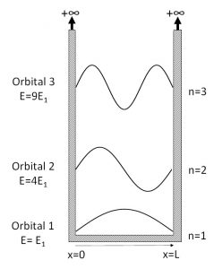
Figure IV.3.A Quantum “particle in a box” model. Wave function shapes and the energy values for the orbitals with the principal quantum number n of 1, 2 and 3 are shown.

Big picture: Developing mathematical descriptions for U(x) for various atoms and molecules belongs to the domain of quantum physics and constitutes a focus of computational chemistry. The models developed by computational chemists need to be verified by experimental spectroscopic measurements (see next chapter) in order to be confirmed and accepted or to be found incompatible with the experimental data and modified or discarded. This process is iterative: currently, many models of U(x) are accepted for various relevant chemical systems while others have been rejected.

QM Example: electrons in a hydrogen atom vs. in a diatomic hydrogen molecule

As the environment for the quantum particle changes, its potential energy U(x) changes as well (that is our models need to take these changes into account). Let’s consider a case of formation of a diatomic H₂ molecule from two isolated hydrogen atoms already discussed in this textbook, see Figure II.3.B. As the di-atomic H₂ molecule forms, the potential energy U(x) for each out of the two electrons changes: from being a part of an atom attracted to just a single nucleus (a single proton), each of these electrons now exist in a di-nuclear molecule being shared (that is influenced) by two nuclei. This is a major change for the potential energy: U(x) is now different and two Molecular Orbitals (MO) now are available for each of the two electrons as opposed to two Atomic Orbitals, AO, available initially for each electron separately. According to the Aufbau principle (recall the General Chemistry material), the two electrons occupy the lowest energy Molecular Orbital, leaving the other one – higher energy MO – unoccupied.

Figure IV.3.B Atomic Orbitals (AO) for isolated hydrogen atoms, Molecular Orbitals (occupied and unoccupied) for an H₂ molecule and their relative energy values. Dashed lines indicate that the MOs are "derived" from specific AOs.

Key result: An exact mathematical description of U(x) for an electron in the field of two nuclei is too complex for the scope of this textbook, so we just see the outcome of the respective modeling and experiments. One key result here is that the energy value for the electrons in the di-atomic H₂ system is lower than the respective value in the isolated H atoms. This explains why bond formation is an exothermic process.

Practice Problems

Practice problem 1. Under the “particle in a box” model, the first orbital (n=1) has its shape similar to that of an S-orbitals in atoms. What can you say about the shape of the second orbital (n=2) predicted by this model? What an actual electron orbital is the second orbital predicted here is similar to in terms of its “shape”?
Hint: take into account that the actual shape of the orbital in the 3D space is described by the square of the wave function.

Practice problem 2. Working within the “particle in a box” model, prove that the wave function represented by equation 3 in this chapter actually works as a solution for differential equation 2 (Schrödinger equation) “within the well” or within an atom.

Practice problem 3. According to the “quantum particle in a box” model, the potential energy outside of the box or well is infinitely high: U(x) = +\(\infty\). What mathematical function describes the wave function outside of the well (or box, or an atom) according to this model? Does this function describe correctly the fundamental fact that an electron stays within the atom and does not venture outside of it?

Practice problem 4*. If one applies the “particle in a box” model to the electron within a hydrogen atom (H), is the distribution of electron energy levels (E_n ∝ n²) consistent with the light emission bands of this atom?