6.1: Prelude to Covalent Bonding

We have examined the basic ideas of bonding, showing that atoms share electrons to form molecules with stable Lewis structures and that we can predict the shapes of those molecules by valence shell electron pair repulsion (VSEPR) theory. These ideas provide an important starting point for understanding chemical bonding. But these models sometimes fall short in their abilities to predict the behavior of real substances. How can we reconcile the geometries of s, p, and d atomic orbitals with molecular shapes that show angles like 120° and 109.5°? Furthermore, we know that electrons and magnetic behavior are related through electromagnetic fields. Both N₂ and O₂ have fairly similar Lewis structures that contain lone pairs of electrons.

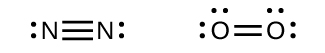
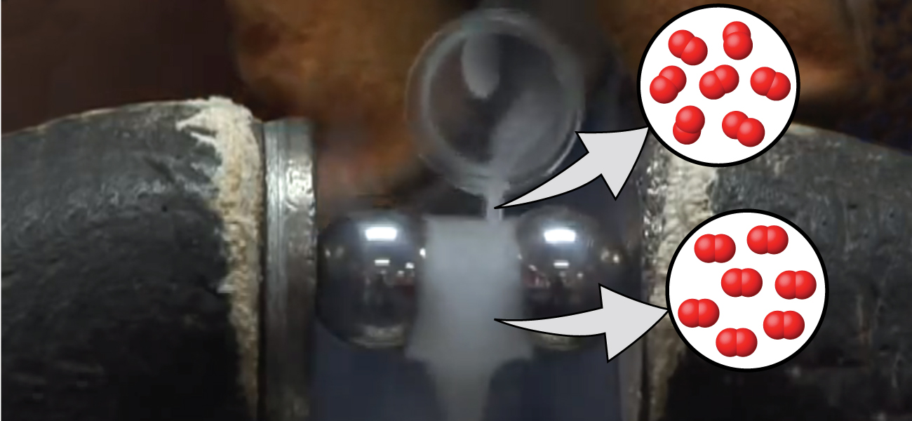
Yet oxygen demonstrates very different magnetic behavior than nitrogen. We can pour liquid nitrogen through a magnetic field with no visible interactions, while liquid oxygen is attracted to the magnet and floats in the magnetic field. We need to understand the additional concepts of valence bond theory, orbital hybridization, and molecular orbital theory to understand these observations.

Figure \(\PageIndex{1}\): Oxygen molecules orient randomly most of the time, as shown in the top magnified view. However, when we pour liquid oxygen through a magnet, the molecules line up with the magnetic field, and the attraction allows them to stay suspended between the poles of the magnet where the magnetic field is strongest. Other diatomic molecules (like N₂) flow past the magnet. The detailed explanation of bonding described in this chapter allows us to understand this phenomenon. (credit: modification of work by Jefferson Lab)

 

Chemical Bonding 

As we know, a scientific theory is a strongly supported explanation for observed natural laws or large bodies of experimental data. For a theory to be accepted, it must explain experimental data and be able to predict behavior. For example, VSEPR theory has gained widespread acceptance because it predicts three-dimensional molecular shapes that are consistent with experimental data collected for thousands of different molecules. However, VSEPR theory does not provide an explanation of chemical bonding.

There are successful theories that describe the electronic structure of atoms. We can use quantum mechanics to predict the specific regions around an atom where electrons are likely to be located: A spherical shape for an s orbital, a dumbbell shape for a p orbital, and so forth. However, these predictions only describe the orbitals around free atoms. When atoms bond to form molecules, atomic orbitals are not sufficient to describe the regions where electrons will be located in the molecule. A more complete understanding of electron distributions requires a model that can account for the electronic structure of molecules.

The energy of the system depends on how much the atomic orbitals of the individual atoms overlap in the geometry of the emolecule. Figure \(\PageIndex{1}\) illustrates how the sum of the energies of two hydrogen atoms (the colored curve) changes as they approach each other. When the atoms are far apart there is no overlap, and by convention we set the sum of the energies at zero. As the atoms move together, their orbitals begin to overlap. Each electron begins to feel the attraction of the nucleus in the other atom. In addition, the electrons begin to repel each other, as do the nuclei. While the atoms are still widely separated, the attractions are slightly stronger than the repulsions, and the energy of the system decreases. (The overall energy is lower than the energy of the individual atoms and thus a bond begins to form.) As the atoms move closer together, the overlap increases, so the attraction of the nuclei for the electrons continues to increase (as do the repulsions among electrons and between the nuclei). At some specific distance between the atoms, which varies depending on the atoms involved, the energy reaches its lowest (most stable) value. This optimum distance between the two bonded nuclei is the bond distance between the two atoms. The molecule is stable because at this point, the attractive and repulsive forces combine to create the lowest possible energy configuration. If the distance between the nuclei were to decrease further, the repulsions between nuclei and the repulsions as electrons are confined in closer proximity to each other would become stronger than the attractive forces. The energy of the system would then rise (making the system destabilized), as shown at the far left of Figure \(\PageIndex{1}\).

Figure \(\PageIndex{1}\): The interaction of two hydrogen atoms changes as a function of distance. The energy of the system changes as the atoms interact. The lowest (most stable) energy occurs at a distance of 74 pm, which is the bond length observed for the H₂ molecule.

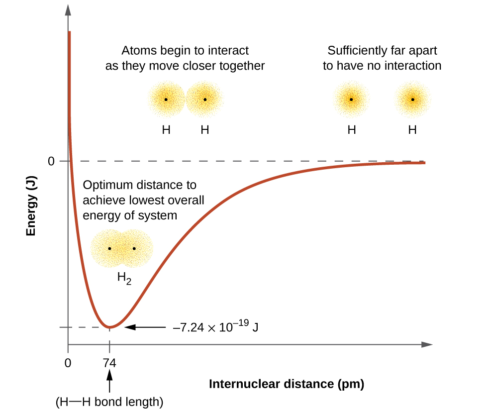
The bond energy is the difference between the energy minimum (which occurs at the bond distance) and the energy of the two separated atoms. This is the quantity of energy released when the bond is formed. Conversely, the same amount of energy is required to break the bond. For the \(H_2\) molecule shown in Figure \(\PageIndex{1}\), at the bond distance of 74 pm the system is \(7.24 \times 10^{−19}\, J\) lower in energy than the two separated hydrogen atoms. This may seem like a small number. However, we know from thermochemistry that bond energies are often discussed on a per-mole basis. For example, it requires \(7.24 \times 10^{−19}\; J\) to break one H–H bond, but it takes \(4.36 \times 10^5\; J\) to break 1 mole of H–H bonds. A comparison of some bond lengths and energies is shown in Table \(\PageIndex{1}\). We can find many of these bonds in a variety of molecules, and this table provides average values. For example, breaking the first C–H bond in CH4 requires 439.3 kJ/mol, while breaking the first C–H bond in \(\ce{H–CH2C6H5}\) (a common paint thinner) requires 375.5 kJ/mol.

Table \(\PageIndex{1}\): Representative Bond Energies and Lengths

Bond	Length (pm)	Energy (kJ/mol)		Bond	Length (pm)	Energy (kJ/mol)
H–H	74	436		C–O	140.1	358
H–C	106.8	413		\(\mathrm{C=O}\)	119.7	745
H–N	101.5	391		\(\mathrm{C≡O}\)	113.7	1072
H–O	97.5	467		H–Cl	127.5	431
C–C	150.6	347		H–Br	141.4	366
\(\mathrm{C=C}\)	133.5	614		H–I	160.9	298
\(\mathrm{C≡C}\)	120.8	839		O–O	148	146
C–N	142.1	305		\(\mathrm{O=O}\)	120.8	498
\(\mathrm{C=N}\)	130.0	615		F–F	141.2	159
\(\mathrm{C≡N}\)	116.1	891		Cl–Cl	198.8	243

 

Attributions

• Modified by Valeria D. Kleiman