
24: Total Spin, Molecules and Molecular Orbital Theory
- Page ID
- 198174
\( \newcommand{\vecs}[1]{\overset { \scriptstyle \rightharpoonup} {\mathbf{#1}} } \)
\( \newcommand{\vecd}[1]{\overset{-\!-\!\rightharpoonup}{\vphantom{a}\smash {#1}}} \)
\( \newcommand{\id}{\mathrm{id}}\) \( \newcommand{\Span}{\mathrm{span}}\)
( \newcommand{\kernel}{\mathrm{null}\,}\) \( \newcommand{\range}{\mathrm{range}\,}\)
\( \newcommand{\RealPart}{\mathrm{Re}}\) \( \newcommand{\ImaginaryPart}{\mathrm{Im}}\)
\( \newcommand{\Argument}{\mathrm{Arg}}\) \( \newcommand{\norm}[1]{\| #1 \|}\)
\( \newcommand{\inner}[2]{\langle #1, #2 \rangle}\)
\( \newcommand{\Span}{\mathrm{span}}\)
\( \newcommand{\id}{\mathrm{id}}\)
\( \newcommand{\Span}{\mathrm{span}}\)
\( \newcommand{\kernel}{\mathrm{null}\,}\)
\( \newcommand{\range}{\mathrm{range}\,}\)
\( \newcommand{\RealPart}{\mathrm{Re}}\)
\( \newcommand{\ImaginaryPart}{\mathrm{Im}}\)
\( \newcommand{\Argument}{\mathrm{Arg}}\)
\( \newcommand{\norm}[1]{\| #1 \|}\)
\( \newcommand{\inner}[2]{\langle #1, #2 \rangle}\)
\( \newcommand{\Span}{\mathrm{span}}\) \( \newcommand{\AA}{\unicode[.8,0]{x212B}}\)
\( \newcommand{\vectorA}[1]{\vec{#1}} % arrow\)
\( \newcommand{\vectorAt}[1]{\vec{\text{#1}}} % arrow\)
\( \newcommand{\vectorB}[1]{\overset { \scriptstyle \rightharpoonup} {\mathbf{#1}} } \)
\( \newcommand{\vectorC}[1]{\textbf{#1}} \)
\( \newcommand{\vectorD}[1]{\overrightarrow{#1}} \)
\( \newcommand{\vectorDt}[1]{\overrightarrow{\text{#1}}} \)
\( \newcommand{\vectE}[1]{\overset{-\!-\!\rightharpoonup}{\vphantom{a}\smash{\mathbf {#1}}}} \)
\( \newcommand{\vecs}[1]{\overset { \scriptstyle \rightharpoonup} {\mathbf{#1}} } \)
\( \newcommand{\vecd}[1]{\overset{-\!-\!\rightharpoonup}{\vphantom{a}\smash {#1}}} \)
\(\newcommand{\avec}{\mathbf a}\) \(\newcommand{\bvec}{\mathbf b}\) \(\newcommand{\cvec}{\mathbf c}\) \(\newcommand{\dvec}{\mathbf d}\) \(\newcommand{\dtil}{\widetilde{\mathbf d}}\) \(\newcommand{\evec}{\mathbf e}\) \(\newcommand{\fvec}{\mathbf f}\) \(\newcommand{\nvec}{\mathbf n}\) \(\newcommand{\pvec}{\mathbf p}\) \(\newcommand{\qvec}{\mathbf q}\) \(\newcommand{\svec}{\mathbf s}\) \(\newcommand{\tvec}{\mathbf t}\) \(\newcommand{\uvec}{\mathbf u}\) \(\newcommand{\vvec}{\mathbf v}\) \(\newcommand{\wvec}{\mathbf w}\) \(\newcommand{\xvec}{\mathbf x}\) \(\newcommand{\yvec}{\mathbf y}\) \(\newcommand{\zvec}{\mathbf z}\) \(\newcommand{\rvec}{\mathbf r}\) \(\newcommand{\mvec}{\mathbf m}\) \(\newcommand{\zerovec}{\mathbf 0}\) \(\newcommand{\onevec}{\mathbf 1}\) \(\newcommand{\real}{\mathbb R}\) \(\newcommand{\twovec}[2]{\left[\begin{array}{r}#1 \\ #2 \end{array}\right]}\) \(\newcommand{\ctwovec}[2]{\left[\begin{array}{c}#1 \\ #2 \end{array}\right]}\) \(\newcommand{\threevec}[3]{\left[\begin{array}{r}#1 \\ #2 \\ #3 \end{array}\right]}\) \(\newcommand{\cthreevec}[3]{\left[\begin{array}{c}#1 \\ #2 \\ #3 \end{array}\right]}\) \(\newcommand{\fourvec}[4]{\left[\begin{array}{r}#1 \\ #2 \\ #3 \\ #4 \end{array}\right]}\) \(\newcommand{\cfourvec}[4]{\left[\begin{array}{c}#1 \\ #2 \\ #3 \\ #4 \end{array}\right]}\) \(\newcommand{\fivevec}[5]{\left[\begin{array}{r}#1 \\ #2 \\ #3 \\ #4 \\ #5 \\ \end{array}\right]}\) \(\newcommand{\cfivevec}[5]{\left[\begin{array}{c}#1 \\ #2 \\ #3 \\ #4 \\ #5 \\ \end{array}\right]}\) \(\newcommand{\mattwo}[4]{\left[\begin{array}{rr}#1 \amp #2 \\ #3 \amp #4 \\ \end{array}\right]}\) \(\newcommand{\laspan}[1]{\text{Span}\{#1\}}\) \(\newcommand{\bcal}{\cal B}\) \(\newcommand{\ccal}{\cal C}\) \(\newcommand{\scal}{\cal S}\) \(\newcommand{\wcal}{\cal W}\) \(\newcommand{\ecal}{\cal E}\) \(\newcommand{\coords}[2]{\left\{#1\right\}_{#2}}\) \(\newcommand{\gray}[1]{\color{gray}{#1}}\) \(\newcommand{\lgray}[1]{\color{lightgray}{#1}}\) \(\newcommand{\rank}{\operatorname{rank}}\) \(\newcommand{\row}{\text{Row}}\) \(\newcommand{\col}{\text{Col}}\) \(\renewcommand{\row}{\text{Row}}\) \(\newcommand{\nul}{\text{Nul}}\) \(\newcommand{\var}{\text{Var}}\) \(\newcommand{\corr}{\text{corr}}\) \(\newcommand{\len}[1]{\left|#1\right|}\) \(\newcommand{\bbar}{\overline{\bvec}}\) \(\newcommand{\bhat}{\widehat{\bvec}}\) \(\newcommand{\bperp}{\bvec^\perp}\) \(\newcommand{\xhat}{\widehat{\xvec}}\) \(\newcommand{\vhat}{\widehat{\vvec}}\) \(\newcommand{\uhat}{\widehat{\uvec}}\) \(\newcommand{\what}{\widehat{\wvec}}\) \(\newcommand{\Sighat}{\widehat{\Sigma}}\) \(\newcommand{\lt}{<}\) \(\newcommand{\gt}{>}\) \(\newcommand{\amp}{&}\) \(\definecolor{fillinmathshade}{gray}{0.9}\)Last lecture address two unique aspects of electrons: spin and indistinguishability and how they couple into describing multi-electron wavefunctions. The spin results in an angular momentum that follows the same properties of orbital angular moment including commutators and the uncertainty effect. The Slater determinant wavefunction was introduced as a way to consistently address both properties.
Remember that the Electronic Configuration is not enough to describe the wavefunction of a multi-Electron Atom
Specification of a particular occupancy of the set of orbitals available to the system gives an electronic configuration. For example,
- \(1s^22s^22p^2\) is an electronic configuration for the carbon atom (and the \(N^{+1}\) and the \(O^{-2} \) ions)
This configuration represents how electrons occupy low-energy orbitals of the system and, as such, are likely to contribute strongly to the true ground and low-lying excited states and to the low-energy states of molecules formed from these atoms or ions.
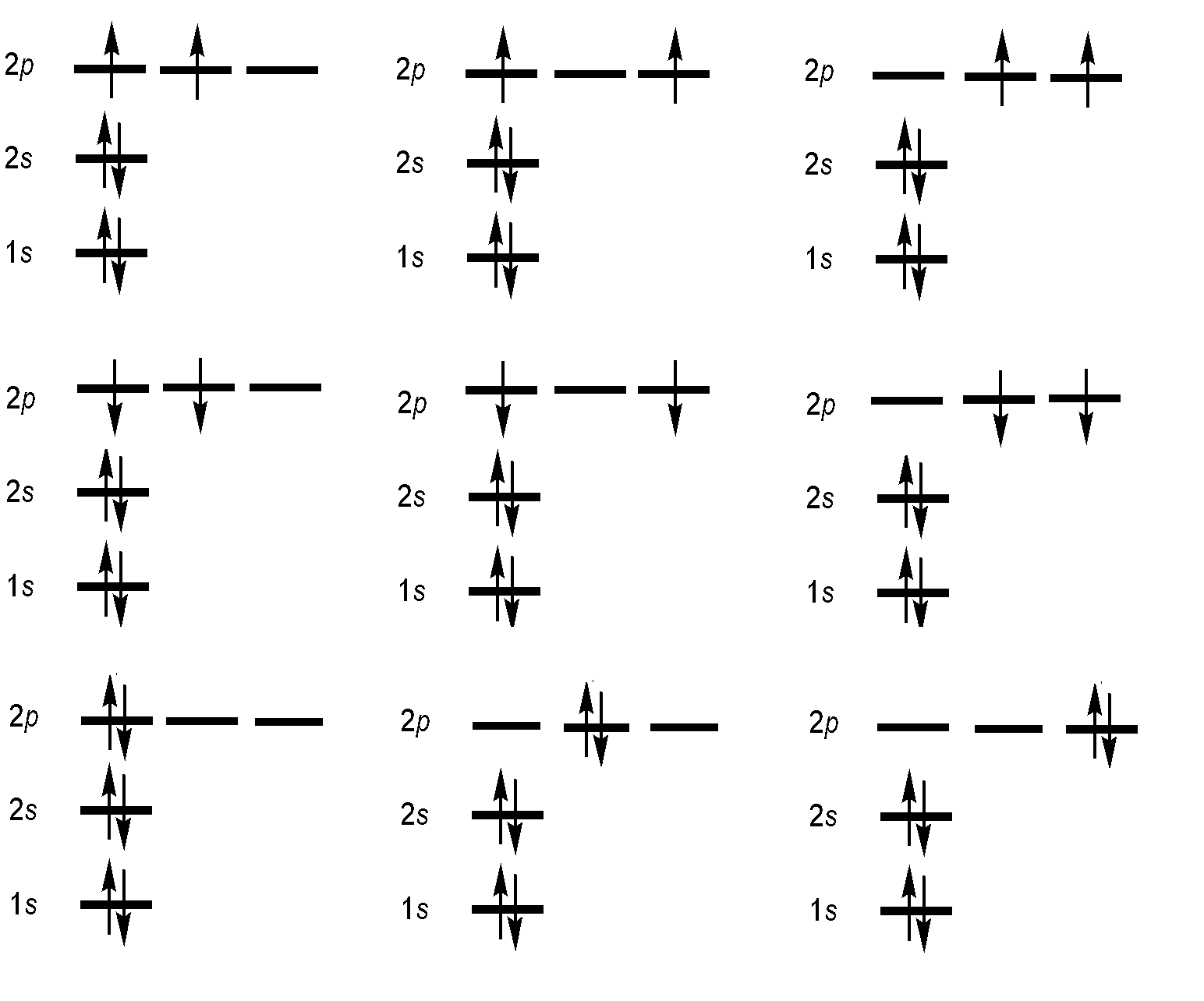
Specification of an electronic configuration does not, however, specify a particular electronic state of the system. For the electronic configuration of carbon with \(1s^22s^22p^2\), there are many ways in which the 2p orbitals can be occupied by the two electrons. As a result, there are a total of multiple "microstates" which cluster into energetically distinct levels, lying within this single configuration.
Specifying the orbital configuration of an atom does not uniquely identify the electronic state!
We want to Couple Angular Momenta to Describe Microstates
Specifying the orbital configuration of an atom does not uniquely identify the electronic state of the atom because the orbital angular momentum, the spin angular momentum, and the total angular momentum are not precisely specified. For example in the 2p electron in Boron can be in any of the three p-orbitals, \(m_l\) = +1, 0, and –1, and have spins with \(m_s\) = +1/2 or –1/2. Thus, there are 3 times 2 different possibilities spin-orbitals this electron can "be in".
Specifying the orbital configuration of an atom does not uniquely identify the electronic state!
The orbital and spin angular momentum of the electrons combine in multiple ways to produce angular momentum vectors that are characteristic of the entire atom not just individual electrons, and these different combinations can have different energies.
Spin-Orbit Coupling (Different Angular Momenta Combinations have different Energies)
The angular momentum manipulations and in particular determining microstates for a specific electron configuration with characteristic term symbols did not suggest these different microstates affected the energy of a multi-electron system. For that to occur the spin must appear in the Hamiltonian.
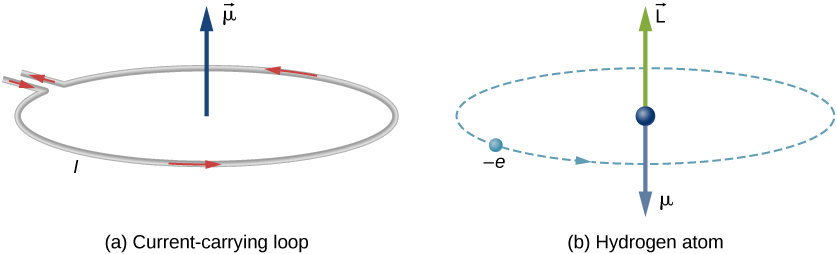
Each type of angular momentum generates magnetic dipoles that interacts:
We have introduced to types of angular momenta in class so far:
- Orbital angular momenta (\(l\)) is the quantum-mechanical counterpart to the classical notion of angular momentum: it arises when a particle executes a rotating or twisting trajectory (such as when an electron orbits a nucleus)
- Spin angular momenta (\(s\)) is an intrinsic form of angular momentum carried by elementary particles. The existence of spin angular momentum is inferred from experiments, such as the Stern–Gerlach experiment.
Quantum numbers for angular momenta in single-electron atoms
The two angular momenta are similarly quantized (both in magnitude and orientation):
\[ |\textbf{L}| = \hbar \sqrt{l(l+1)}, \quad L_z = m_l \hbar \]
\[ |\textbf{S}| = \hbar \sqrt{s(s+1)}, \quad S_z = m_s \hbar\]
where
- \(l\), is the azimuthal quantum number,
- \(s\), is the spin quantum number intrinsic to the type of particle,
For orbital angular momenta, the eigenvalues for \(L^2\) and \(L_z\) are quantified (naturally)
\[ \hat{L^2} \,|Y_{l\,m} \rangle = l\,(l+1)\,\hbar^2\, |Y_{l\,m} \rangle\]
where \(l\) is an integer. The eigenvalue for spin angular momenta (of an electron) the \(s\) quantum number is only either +1/2 or -1/2
\[ \hat{S^2} \,| spin \rangle = s\,(s+1)\,\hbar^2\, | spin \rangle \]
Quantum numbers for angular momenta in single-electron atoms
The angular momentum of \(N\) particles is the vector sum of constituent particles
\[ \vec{L} = \sum_i^N \vec{l}_i\]
and the z-component of is the scalar sum
\[ L_z = \sum_i^N L_{z,i}\]
The spin momentum of \(N\) particles is the vector sum of constituent particles
\[ \vec{S} = \sum_i^N \vec{s}_i\]
and the z-component of is the scalar sum
\[ S_z = \sum_i^N S_{z,i}\]
Angular Momentum (Spin and Orbital) Multiplicity
Quantum mechanics states that the component of angular momentum measured along any direction can only take on the values
\[ L_z = \hbar m_l\]
with
\[m_l \in \{ - l, -(l-1), \dots, 0, \ldots, l - 1, l \} \]
where \(L_z\) is the spin component along the z-axis, \(m_l\) is the spin projection quantum number along the z-axis. One can see that there are \(2L+1\) possible values of \(L_z\). The number "2L + 1" is the multiplicity of the spin system (referred to this as degeneracy before).
So the multiplicity of state with orbital angular momenta \(L\)
\[2L+1\]
and for spin angular momenta \(S\)
\[2S+1\]
Notice that these equations involve BIG \(L\) for all electrons in the atom, not \(l\) for one electron. The same for spin.
How many possible states are there for a single spin-1/2 particle (e.g. electron) with \(m_s = +1/2\) and \(m_s = −1/2\).)?
- Answer
-
The spin multiplicity of a single electron is
\[2S+1 = 2 (1/2) +1 =2 \]
These correspond to quantum states in which the spin is pointing in the +z or −z directions respectively, and are often referred to as "spin up" and "spin down".
Compare this for a spin-3/2 particle (which exist), the multiplicity is \(2S+1 = 2 (3/2) +1 = 4\). So the possible values of \(m_s\) are +3/2, +1/2, −1/2, −3/2. This is important for NMR spectroscopy, by the way.
There are only two possible values for a spin-1/2 particle like the electron. This is not surprising.
What about a two-electron system?
- Answer
-
For a two electron system each electron can occupy two states (four total), but due to indistinguishability, these are really two states
- ½ and ½ (aligned spins)
- ½ and - ½ (opposed spins)
which correspond to
\( S = ½ + ½ = 1\) and \(S= ½ - ½ = 0\)
The multiplicity of these two states (\(2S+1\)) are then
For \(S =1\):
\[2S+1 = 3 \nonumber\]
This is called a triplet state since there are actually three states (commonly called microstates) that represent this state
For \(S=0\):
\[2S+1 = 1 \]
This is called a singlet state since only one state represents it.
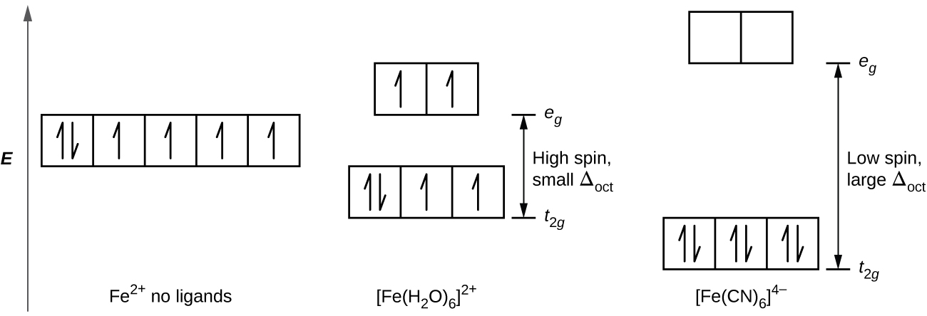
It should be noted that for multi-electron systems where all electrons are paired, the system is in a singlet. Also note that singlets are diamagnetic, while triplets are paramagnetic.
You probably learned about paramagnetism and diamagnatism in general chemistry, specifically crystal field theory
The Born-Oppenheimer Approximation
We will consider a very general molecule with \(N\) nuclei and \(M\) electrons. The coordinates of the nuclei are \(R_1 ,...,R_N\). The coordinates of the electrons are \(r_1 ,...,r_M\), and their spin variables are \(S_{z,1},...,S_{z,M}\). For shorthand, we will denote the complete set of nuclear coordinates as \(R\) and the set of electrons coordinates as \(r\) and \(x\) the complete set of electron coordinates and spin variables. The total molecular wave function \(\psi (x,R)\) depends on \(3N+4M\) variables, which makes it a very cumbersome object to deal with. The Born-Oppenheimer approximation leads to a very important simplification of the wave function.
Nuclei move and electrons adjust quickly.
If we could neglect the electron-nuclear interaction, then the wave function would be a simple product \(\psi (x,R)=\psi_{elec}(r)\psi_{nucl}(R)\). However, we cannot neglect this term, but it might still be possible to write the wave function as a product. We note, first, that most nuclei are 3-4 orders of magnitude heaver than an electron. For the lightest nucleus, the proton,
\[m_p \approx 2000 m_e\]
This mass difference is large enough to have important physical consequences. Let us think classically about this mass difference first. If two particles interact in some way, and one is much heavier than the other, the light particle will move essentially as a "slave'' of the heavy particle. That is, it will simply follow the heavy particle wherever it goes, and, it will move rapidly in response to the heavy particle motion.
Considering this as a classical system, we expect that the motion will be dominated by the large heavy particle, which is attached to a fixed wall by a spring. The small, light particle, which is attached to the heavy particle by a spring will simply follow the heavy particle and execute rapid oscillations around it.
So a good approximation is to describe the electronic states of a molecule by thinking that the nuclei are not moving, i.e. that they are stationary. The nuclei, however, can be stationary at different positions so the electronic wavefunction can depend on the positions of the nuclei even though their motion is neglected.
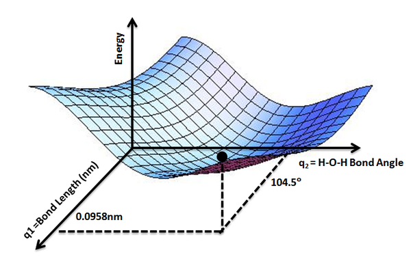
The Born-Oppenheimer Approximation gives us the Concept of a Potential Energy Curve or Surface
In practice the electronic Schrödinger equation is solved using approximations at particular values of \(R\) to obtain the wavefunctions \(\varphi _e (r,R)\) and potential energies \(V_e (R)\).
While the potential energy function, \(V_e (R)\), for a diatomic molecule is a 1-D curve, molecules with more than two atoms will have multi-dimensional potential energy surfaces with 3N-6 (or 3N-5 for linear molecule) dimensions for the number of internal degrees of freedom.
The mass of an electron is 1860 times less than that of a proton. This is a crucial difference since it permits us to treat the electrons as a wave function while treating the nuclear positions as fixed. In effect, the nuclei are not being treated using the wave-like properties. If they were then we would need to solve two simultaneous wave equations in order to describe even the simplest atom. The mass difference also leads to a difference in time scale for motion, which is the fundamental physical reason that the approximation holds.
The \(H_2^+\) ion and Hydrogen Molecule
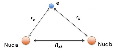
\[\hat {H}_{elec} (r, R_{ab}) = -\dfrac {\hbar ^2}{2m} \nabla_a ^2 -\dfrac {\hbar ^2}{2m} \nabla_b ^2 -\dfrac {\hbar ^2}{2m} \nabla ^2 - \dfrac {e^2}{4 \pi \epsilon _0 r_a} - \dfrac {e^2}{4 \pi \epsilon _0 r_b} + \dfrac {e^2}{4 \pi \epsilon _0 R_{ab}} \label{H2+}\]
where
- \(r_a\) and \(r_a\) are the distances electron from the \(a\) and \(a\) hydrogen nuclei, respectively and
- \(R_{ab}\) is the distance between the two protons.
If we invoke the Born Oppenheimer approximation (i.e., fix the nuclear motion), we can drop the kinetic energy terms of the nuclei (notice semi-colon to represent that the wavefunction depends parametrically on the geometry (\(R\)) of the system instead as an explicit variable in the system like \(r_1\))
\[\hat {H}_{elec} (r; R_{ab}) = \underbrace{-\dfrac {\hbar ^2}{2m} \nabla ^2}_{\text{KE}} \underbrace{- \dfrac {e^2}{4 \pi \epsilon _0 r_a}}_{\text{Attract}}\underbrace{ - \dfrac {e^2}{4 \pi \epsilon _0 r_b}}_{\text{Attract}} + \underbrace{\dfrac {e^2}{4 \pi \epsilon _0 R_{ab}}}_{\text{repel/constant}} \]
This can be solved though since it is not a three-body system (only one particle is moving). What about for the hydrogen molecule?
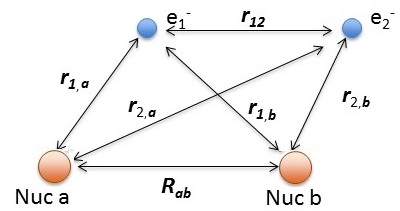
The relevant Hamiltonian (within BO approximation with fixed nuclei) is
\[\hat {H}_{elec} (r; R_{ab}) = -\dfrac {\hbar ^2}{2m} \nabla_1 ^2 -\dfrac {\hbar ^2}{2m} \nabla_2^2 - \dfrac {e^2}{4 \pi \epsilon _0 r_{1,a}} - \dfrac {e^2}{4 \pi \epsilon _0 r_{1,b}} - \dfrac {e^2}{4 \pi \epsilon _0 r_{2,a}} - \dfrac {e^2}{4 \pi \epsilon _0 r_{2,b}} + \dfrac {e^2}{4 \pi \epsilon _0 r_{12}} +\underbrace{\dfrac {e^2}{4 \pi \epsilon _0 R_{ab}}}_{\text{repel/constant}}\]
using the distances defined above.
We can analytically solve the \(H_2^+\) system (within the Born-Oppenheimer approximation), but we often do not in physical chemistry courses, since the solutions are not applicable to multi-electron diatomics. That requires an approximation like that discussed below.
The Linear Combination of Atomic Orbitals (LCAO) Approximation
First we will extend the orbital approximation from atoms to molecules, so the general multi-electron wavefunction in a molecule (at a specific configuration of nuclei, \(R\)) is
\[ | \psi (r_1, r_2, r_3 .. r_n; R) \rangle \approx | \phi_1 (r_1; R) \phi_2 (r_2; R) \phi _3(r_3; R) ... \phi_n (r_n; R) \rangle \label{wrong}\]
where \(\phi_n (r_n; R) \) are molecular orbitals (constructed with a specific configuration of \(R\)).
Equation \(\ref{wrong}\) is an incorrect formulation of the true multi-electron molecular wavefunction since it is an orbital approximation.
We can expand each molecular orbital into any complete basis. The one that we choose here is the basis of all atomic orbitals on all nuclei. So
\[ \phi_i (r ; R ) = \sum _{k=1}^N \sum_{j}^{j= \infty} a_{j,k} |AO_{j,k} \rangle \label{LCAO}\]
where
- \(i\) is the index for the \(i^{th}\) molecular orbital
- \(j\) is the index for the \(j^{th}\) atomic orbitals on the \(k^{th}\) nucleus
- and \(a_{j,k}\) is the coefficient representing the amplitude (and sign) of the \(j^{th}\) atomic orbital on the \(k^{th}\) nucleus in the expansion.
To be a complete basis, this expansion must include all possible atomic orbitals, which is not numerically feasible of course. But only certain orbitals dominate the expansion (sort of like perturbation theory expansions discussed before).
This is called the Linear Combination of Atomic Orbital (LCAO) approximation for describing molecular orbitals.
The \(H_2^+\) molecular cation
The LCAO approximation is a simple method of quantum chemistry that yields a qualitative picture of the molecular orbitals in the hydrogen diatomic molecules.
\[| \phi (r) \rangle = C_A 1s_A (r) + C_B1s_B (r)\]
We must determine the values for the coefficients, \(C_A\) and \(C_B\). We could use the linear variational method to find a value for these coefficients, but for the case of H2+ evaluating these coefficients is easy. Since the two protons are identical, the probability that the electron is near nucleus \(A\) must equal the probability that the electron is near nucleus \(B\). These probabilities are given by \(|C_A|^2\) and \(|C_B|^2\), respectively.
more next lecture
Last lecture addressed the consequence of indistinguishability in electronic structure calculations. The Hartree and Hartree-Fock (HF)caclulations were introduced within the Self-Consistent-Field (SCF) approach (similar to numerical evaluation of minima). The Hartree method treats electrons via only as an average repulsion energy and the HF approach using Slater determinant wavefunctions introduces an exchange energy term. Ionization energy and electron affinities are discussed within the context of Koopman's theorem.