10.6: Diffusion and Effusion

Diffusion

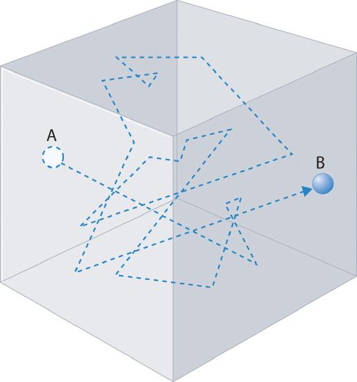
Diffusion is how a gas disperses through space and is the result of the random motion as illustrated in Figure \(\PageIndex{1}\). The gas follows the postulates of the Kinetic Molecular Theory, moving like a classical particle and changing directions every time there is a collision. Note a typical gas molecule has in the order of 10¹⁰ collisions per second and the distance between collisions is the mean free path.

Figure \(\PageIndex{1}\): Random path a particle takes as it traverses a container.

The following YouTube gives a good demonstration of diffusion and effusion.

Video \(\PageIndex{1}\): (4:00 YouTube). Note, at 1:22 they show the diffusion of gas into a vacuum, while at 1:51 the same gas diffuses into a container with air. At 2:36 there is a good example involving HCl and NH₃ demonstrating Grahm's Law of Effusion.

Effusion

Effusion is related to diffusion and is how a gas escapes through a hole in one container into another (evacuated) container.

Figure \(\PageIndex{2}\): demonstrating effusion, note the lighter helium effuses fastere than the heavier ethylene oxide.

The Scottish chemist Thomas Graham measured the effusion rates of gases at constant temperature and discovered that they were inversely proportional to the square root of the molar mass.

\[\mathrm{Rate \; of \; effusion} \propto \frac{1}{\sqrt{\mathfrak{M}}}, \; \mathfrak{M}=Molar \; Mass\]

This results in the common relationship known as Graham's Law

\[\dfrac {\it{Rate\;of\;effusion\; of \;A} }{ \it{Rate \;of \;effusion\; of \;B}}=\dfrac{(u_{rms})_A}{(u_{rms})_B}=\dfrac{\sqrt{\mathfrak{M}_B}}{\sqrt{ \mathfrak{M}_A}}\]

Which can be derived from KMT and ideal gases (last section of 10.5)

\[ u_{rms}=\sqrt{\frac{3RT}{\mathfrak{M}}}\]

Where,

\[\dfrac {\it{Rate\;of\;effusion\; of \;A} }{ \it{Rate \;of \;effusion\; of \;B}}=\dfrac{(u_{rms})_A}{(u_{rms})_B}=\dfrac{\sqrt {3RT\mathfrak{M}_A}}{\sqrt{3RT/\mathfrak{M}_B}}=\dfrac{\sqrt{\mathfrak{M}_B}}{\sqrt{\mathfrak{M}_A}}\]

A simple way to remember this is to remember postulate 5 of KMT, which states that the kinetic energy of a gas is proportional to the absolute temperature and then equate the average kinetic energy of two gases

\[e_K=\dfrac{1}{2}m{u_{rms}^2}\]

so,

\[e_K= (\dfrac{1}{2}m{u_{rms}^2})_A= (\dfrac{1}{2}m{u_{rms}^2})_B\]

which rearranges to the above relationship

\[\dfrac{(u_{rms})_A}{(u_{rms})_B}=\dfrac{\sqrt{\mathfrak{M}_B}}{\sqrt{\mathfrak{M}_A}} \; \; \; or \; \; \; \dfrac{(u_{rms})^2_A}{(u_{rms})^2_B}=\frac{\mathfrak{M}_B}{\mathfrak{M}_A} \]

Trick:

If a gas were a particle, you could say the kinetic energy of the particle of gas is \(\frac{1}{2}mv^2\) and you could equate to kinetic energies of two gas particles as

\[\frac{1}{2}m_1v_1^2 = \frac{1}{2}m_2v_2^2\]

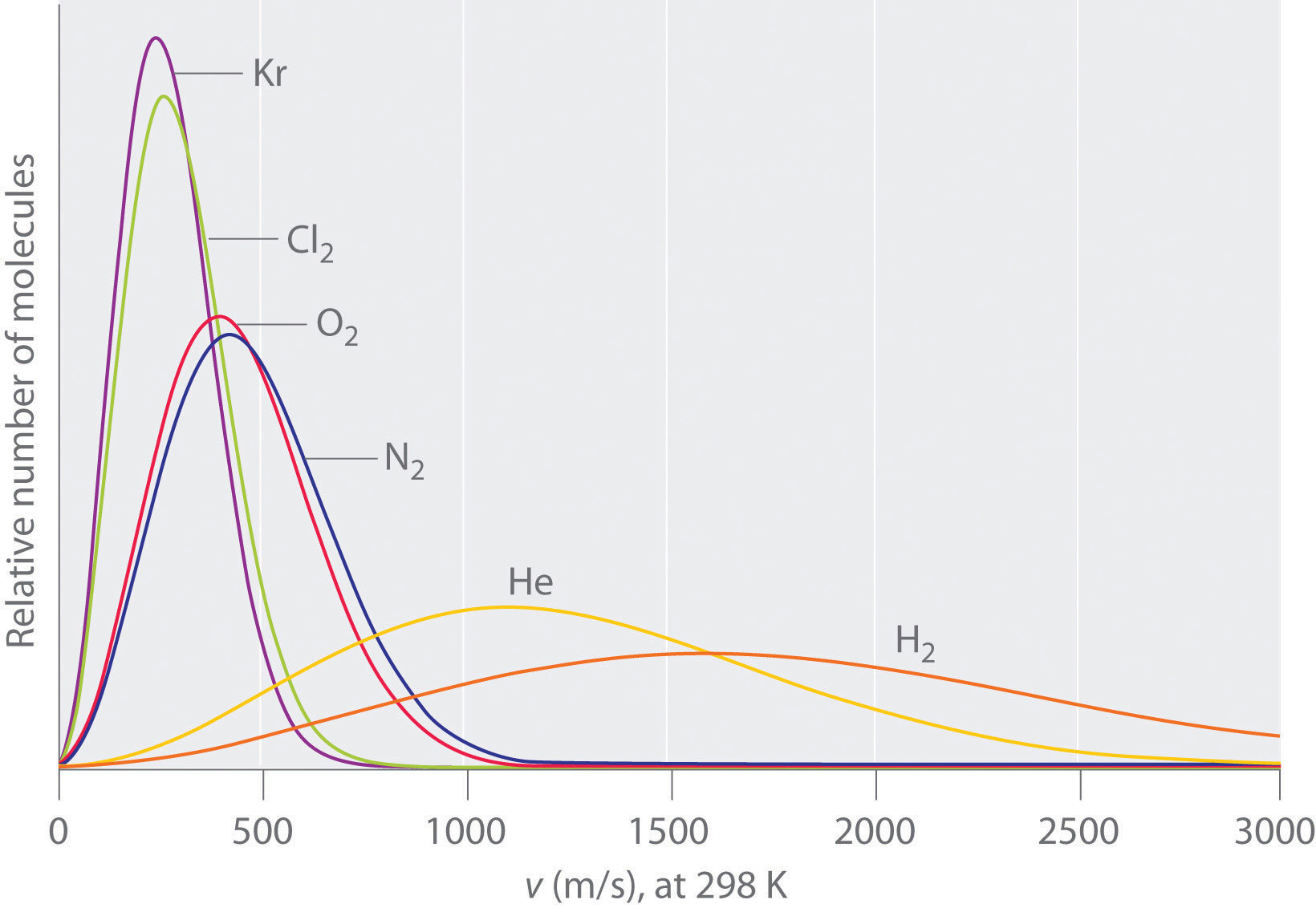
Now the above equation does NOT represent a gas, which has many particles possessing a range of velocities, like those in Figure \(\PageIndex{3}\), but it has the same form as equation 10.6.6. The difference is if the particles represent different chemicals, the mass is the molar mass, and you use the root mean square velocity for a gas, instead of the velocity of a single particle. So this may help you remember the equation.

Since gasses at the same temperature have the same kinetic energy the energy profile plots skew to the right for small molecules (that have small m and large v), while heavy molecules (larger m) have smaller velocities.

Figure \(\PageIndex{3}\): Velocity profiles for different gasses at the same temperature. note the average kinetic energy is the same, and so the lighter molecules tend to travel faster.

Example \(\PageIndex{1}\): Graham's Law Problem

Ammonia and nitric acid are swabbed onto cotton and placed at the ends of a 1 meter evacuated tube, like is done at 2:36 in the above youTube (video 10.6.1). How far from the ammonia side does the ammonium nitrate form?

Video \(\PageIndex{2}\)