3.2: Solutions and Freezing Point Depression

 

Learning Objectives

Goals: 

• Collect experimental data and express concentration in different units.
• Observe the concentration dependence on the colligative effect of freezing point depression
• Observe the challenges of experimental measurements and importance of equipment calibration
• Understand the challenge of science by trying to determine the Van't Hoff factor for two different concentrations of sodium nitrate

By the end of this lab, students should be able to:

• Use a volumetric flask to make a solution
• Know the precision of volumetric flasks and perform calculations to the correct number of significant digits.
• Demonstrate an understanding of the colligative propertiy of freezing point depression

Prior knowledge:

• Solutions (section 4.4)
• Intermolecular Forces (chapter 11)

Concurrent Reading

• Units of Concentration (section 13.1)
• Colligative Properties (section 13.4)

 

Safety

• Emergency Preparedness
  • Eye protection is mandatory in this lab, and you should not wear shorts or open toed shoes. 
  • NaCl PubChem LCSS
• Minimize Risk
  • Never place dry ice in sealed container.
  • Never touch the dry ice as it can cause frostbite, and do not play around with it. 
  • Do not pour water into calorimeter containing dry ice, it could form an ice seal that traps the dry ice and could splatter ice particles.

Video\(\PageIndex{1}\): 3:25 min video on hazards with dry ice by Science of Lab Safety (https://youtu.be/qJSSTUru2MQ)

 

• Recognize Hazards
  • Do not use alcohol thermometers
  • Dispose of waste as instructed

 

 

Equipment and materials needed

25 mL volumetric flask	analytical balance	NaCl(s)
dry ice (solid CO2)	ice (solid water)	2 250 mL Erlenmeyer Flask
eye dropper	Vernier LabQuest	Temperature Probe
two 8 in test tube	stirrer	calorimeter
leather gloves	tongs

 

Background

There are two parts to this experiment.  In the first part, you will make two different aqueous solutions of sodium chloride and express their concentration in different ways.  Then you will place the solutions in a calorimeter containing dry ice and solidify around 20% of the water in the salt water solution and then measure the temperature at which the last bit of ice melts, and record this as the freezing point of the ice solution

The first part of this experiment is routine and the "work" is in the write up, where you need to express your solutions in multiple units.  The second part is far more challenging, but if you do your work carefully you can get real good data with the equipment we are using.  But, you can also get real bad data if you are not careful.

Part 1: Solutions

In this part of the experiment you will make two solutions of sodium chloride and report their concentrations in different units (sec. 13.1). You will add some solid salt to a 25 mL volumetric flask and dilute to volume (add water until the meniscus aligns with the calibration mark). A common mistake is to make that measurement while there is still solid (undissolved) salt in the flask.  If you can not dissolve all the salt you have a saturated solution and you have no idea what the concentration is, because you do not know how much is at the bottom (think about experiment 2). But even if you can dissolve it all, you need to double check the volume after mixing as there if often a contraction in volume upon mixing, especially if you are dissolving ionic compounds in water. 

This is because the ion-dipole forces (sec. 11.2) of the solute-solvent interactions are often stronger than the dipole/hydrogen bonding forces between water molecules, so the water is pulled in closer to the ions than it is pulled to itself, resulting in a contraction in the total volume upon mixing.  So you add the salt to the volumetric flask, fill it half way and try and mix it so all the solid dissolves.  Then you dilute it to volume.  But no matter what, make sure all the solute is dissolved before you make your final volumetric measurement.

You will save these solutions for the second part of the lab.

Part 2: Freezing Point Depression

Colligative properties (sections 3.4.3-3.4.6 ) are properties of a solvent that a solute affects, like the freezing or boiling point of the solvent.  In this lab we will measure the freezing point of the two solutions created in the first part of the lab and compare them to pure water.  You should observe that as the salt concentration increases the freezing decreases, and this can be explained by the following equation:

\[\begin{align} \Delta T & =-ik_{f}m  \\ &\text{where} \nonumber \\ i & = \text{Van't Hoff Factor} \nonumber \\ k_{f} & = \text{cryoscopic (melting point depression) constant} \nonumber \\ m & = \text{molality} \left ( \frac{mole_{solute}}{kg_{solvent}} \right ) \nonumber  \\ & and \nonumber   \\ \nonumber \Delta T & = T_{fp}\text{(solution)}-T_{fp}\text{(pure solvent)} \nonumber \end{align}\]

The value of k_f for various solvents can be obtained from table 13.4.2.

For a non-electrolyte i=1 and the Van't Hoff equation is expressed as: 

\[\Delta T  =-k_{f}m \]

Note

If the value of k_f from a thermodynamic table is negative, remove the negative sign from the above equation (use  \(\Delta T =ik_{f}m\) if k_f is a negative). That is, the freezing point is always depressed, and some table report these as positive values and others as negative values.  So be alert!

What is confusing for many people is that the Van't Hoff factor (i) is itself a function of the molality (section 13.4.5).  The Van't Hoff factor (i) takes into account the dissociation of ionic compounds upon dissolution and is the number of ions in an ionic formula for an "ideal solution." This value is approached for dilute solutions, but as the solute becomes more concentrated the solute particles interact with each other and the observed value of i is less than the number of particles the ionic compound breaks into.  The value of i can be experimentally determined by comparing the observed \(\Delta T\) with the predicted  \(\Delta T\) if the ionic compound was considered to be a nonelectrolyte (i=1).

given

\[\begin{align} & \Delta T_{real} =ik_{f}m \nonumber \\   & \;\;\;\;\;\;\;\; and \nonumber \\  &\Delta T_{\text{i=1, nonelectrolyte}}  =-k_{f}m\end{align}\]

where the second term is not taking into account the ions the solute breaks into.  If we divide the first by the second we get:

\[\frac{\Delta T_{real}}{\Delta T_{i=1}}=\frac{ik_fm}{k_fm}\]

so

\[i=\frac{\Delta T_{real}}{\Delta T_{i=1}}\]

That is, we simply divide the observed temperature depression by that which we would get if we did not take into account the dissociation of the ionic compound.

There are two major problems with measuring the freezing point of a salt water mixture.  First, is freezing the substance and second, is that the moment some of the water freezes the concentration of the salt in the liquid phase goes up, and so the freezing point goes down.  The video in section 13.4.4 shows how the freezing point depression results from the solute interfering with the growth of the crystal, which are essentially pure water (although salt particles do get trapped in the crystal, most likely in the interstitial regions). A consequence is that pure water has a constant temperature as it goes from pure liquid to pure solid, while salt water does not.  So if you froze a container of pure water the temperature would be the same if it was 90% water/10% ice or 10% water/90% ice. In contrast a salt water mixture water would be warmer when it was 90% salt water/10% ice and colder when it was 10% salt water/90% ice.  An interested biological effect of this is that there are lateral bands in polar sea ice of brine (salt water) channels that support a subzero ecosystem complete with brown photosynthetic algae that migrate vertically up and down the ice pack due to seasonal temperature variations (figure \(\PageIndex{1}\), NOAA PMEL Artic Zone).

 

 

Figure \(\PageIndex{1}\): Band of brown sea ice algae living in salt water (brine) channels in Artic sea ice. Near the surface the temperature can get down to -35^oC while deeper down it warms up, and living organisms can live in the brine channels when the temperatures are above -5^oC. The salinity of the channels changes as the temperature changes and so there are bands that the brown photosynthetic organisms can live in, and these migrate up and down the ice pack due to seasonal temperature changes.  It is estimated that sea ice algae are responsible for up to 57% of the primary photosynthetic production in the artic and the brown pigments are due to spectral changes of the light as it passes through the ice pack (see PMEL Artic Zone) (Copyright; Artic Zone, Pacific Marine Environmental Laboratory, NOAA)

It would be nice if we had a sub-zero freezer with a watch glass that allowed us to control and observe the temperature at which the salt solution freezes, but we do not have one.  So we are going to use an endothermic reaction to cool the solution down, the sublimation of solid carbon dioxide.  We will place the salt water in an 8 in test tube and then put the test tube in thermal contact with dry ice. The problem is that at 1 atm dry ice sublimes at -78.5^oC and so will very quickly the salt water.  You will place a digital thermometer into the salt water solution and then place in an open calorimeter that has some dry ice shavings.  The temperature will cool very rapidly until the solution starts to freeze, and you want to freeze about 10% of the solution, and then pull it out of the cold calorimeter and place in an Erlenmeyer flask. Initially the ice will be at the bottom of the test tube, where it was in contact with the dry ice, and that part of the test tube will be colder than the rest. You need to stir the solution and make sure the ice floats to the top before it melts and record the temperature when the last piece of ice melts.  You can only know the molality when the last bit of ice melts and you need to be sure you have a constant temperature throughout the solution when you record that measurement, so it is imperative that you stir the solution while you are melting the ice.  If done with care, you can get very accurate data, but it is tricky.

Experimental Procedures

Part 1: Preparing solutions

Solution 1

1. Weigh an empty 25 mL volumetric flask and record the mass in your data sheet to the precision of your instrument
2. Weigh approx 0.5 g sodium chloride and add to the 25 mL volumetric flask.
3. Weigh the flask with the solid solute and record the mass in your data sheet to the precision of your instrument
4. Fill the flask a bit over half way to mark with deionized water and swirl to dissolve all the solute. Continue filling to mark, using an eye dropper to add the last few drops.  Be sure all the solute is dissolved
5. Weigh the volumetric flask with aqueous salt solution and record the mass in your data sheet to the precision of your instrument
6. Pour the solution from the volumetric flask into a 100 mL beaker labeled #1 and set aside.  You will use it in part 2.
7. Clean the volumetric flask with DI water.  You do not need to dry it.

Solution 2

1. Repeat steps 1-5 for solution 1 but use approximately 3 g of NaCl.
2. Pour solution into 100 mL beaker labeled #2 and set aside. You will use it in part 2.

Part 2: Freezing point determination

1. Obtain a Vernier LabQuest, hook up the temperature probe and set it to "meter" with the scale reading in ^oC.  Instructions for running the LabQuest are in the Instrumentation section of your lab manual (sections 0.4.1 & 0.4.2).
2. Fill a 150mL beaker about 1/3 full with ice, pour water over it, insert temperature probe into ice water and once the temperature stabilizes record the temperature of the pure water and ice mixture.
3. Place about 10 mL of solution #1 into the 8 in test tube and insert digital temperature probe. Keep test tube in an empty Erlenmeyer flask when not using.
4. Add a small amount of dry ice to the bottom of calorimeter and insert 8 in test tube with solution 1 and temperature probe into calorimeter.  
5. Observe the temperature decrease until it stabilizes, which will occur when the salt solution begins to form ice, remove test tube from calorimeter and place in the ice water beaker, stirring with temperature probe (This slows down the warming so you have more time to observe).  Be sure the ice floats to the top.
6. Record the temperature the moment the last bit of ice melts. This will be considered the freezing point of the solution of the salt concentration you made.
7. Using a second 8 in test tube repeat steps 3-6 for solution #2.
8. Have instructor check data
9. Repeat trial for all solutions if instructed(you can use the same test tubes and solution)
10. Place waste in waste container and clean up your work station.

 

 

Data Analysis

In this lab you will work your data up in a Google Spreadsheet, the template of which can be downloaded on the report page (3.3A: Solutions and Freezing Point Depression Report). There are three sheets in the Google Workbook

Cover page tab

The first tab is always the cover page.  Please fill it out.

Solutions tab

 

Figure \(\PageIndex{1}\): Transfer the data from your data sheet to the red area, and the answers to your calculations in the blue area (CC0-Belford/Poirot)

 

Temperature tab

The goal of this experiment is to calculate the actual Van't Hoff Factor of a salt solution in the lab. Use the background information above to assist with how to set up ratio to find the real i.

Remember to use freezing points actually observed in the lab, not theoretical values.

The freezing point depression constant can be found in the Resources tab of any LibreText page (Resources/Reference tables/reference tables/bulk properties/cryoscopic/Melting Point Depression constants) or section 13.4.3.1.  But you should become familiar with the blue resources tab on the left of all LibreText pages, as the function like the appendices in a normal textbook.

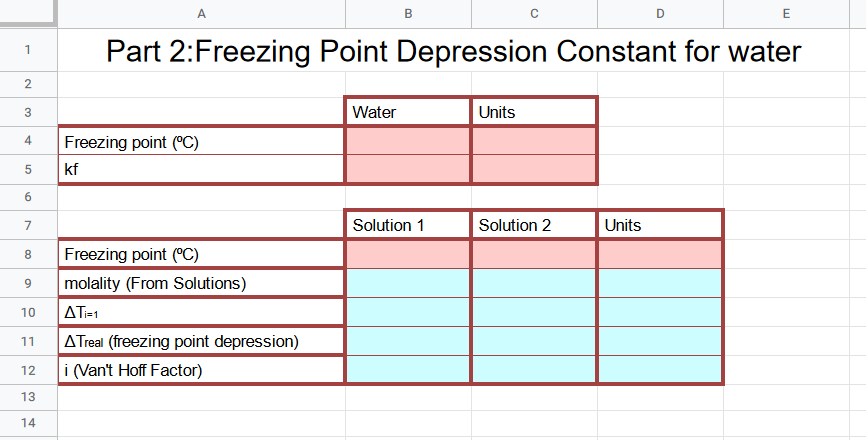Figure \(\PageIndex{2}\): Transfer the data from your data sheet to the red area, and the answers to your calculations in the blue area (CC0-Belford/Poirot)

Note

If you use ΔT=iKfm then you say ΔT=Tsolvent+Tsolution
If you use the ΔT=-iKfm then you say ΔT=Tsolution-Tsolvent

Freezing point (⁰C) Water: The freezing point of water you observed in the lab

Kf: Freezing point constant of solvent (from table)

For solution 1 and 2

Enter the freezing point observed for each solution in the lab

Copy the molality calculated in the solutions tab

Solve for the van't hoff factor using the Freezing Point Depression Equation, Rows 10 and 11 help show your work for solving for i

ΔTi=1 is the theoretical delta T if the van't hoff factor was 1, so ΔTi=1=Kfm