8.5: Extraction Theory

Partition/Distribution Coefficient \(\left( K \right)\)

When a solution is placed in a separatory funnel and shaken with an immiscible solvent, solutes often dissolve in part into both layers. The components are said to "partition" between the two layers, or "distribute themselves" between the two layers. When equilibrium has established, the ratio of concentration of solute in each layer is constant for each system, and this can be represented by a value \(K\) (called the partition coefficient or distribution coefficient).

\[K = \dfrac{\text{Molarity in organic phase}}{\text{Molarity in aqueous phase}}\]

For example, morphine has a partition coefficient of roughly 6 in ethyl acetate and water.\(^2\) If dark circles represent morphine molecules, \(1.00 \: \text{g}\) of morphine would distribute itself as shown in Figure 4.11.

Figure 4.11: Distribution of morphine in ethyl acetate and water.

Note that with equal volumes of organic and aqueous phases, the partition coefficient represents the ratio of particles in each layer (Figure 4.11a). When using equal volumes, a \(K\) of \(\sim 6\) means there will be six times as many morphine molecules in the organic layer as there are in the water layer. The particulate ratio is not as simple when the layer volumes are different, but the ratio of concentrations always equals the \(K\) (Figure 4.11b).

The partition coefficients reflect the solubility of a compound in the organic and aqueous layers, and so is dependent on the solvent system used. For example, morphine has a \(K\) of roughly 2 in petroleum ether and water, and a \(K\) of roughly 0.33 in diethyl ether and water.\(^2\) When the \(K\) is less than one, it means the compound partitions into the aqueous layer more than the organic layer.

Choosing a Solvent with Solubility Data

The partition coefficient \(K\) is the ratio of the compound's concentration in the organic layer compared to the aqueous layer. Actual partition coefficients are experimental, but can be estimated by using solubility data.

\[\begin{align} K &= \dfrac{\text{Molarity in organic phase}}{\text{Molarity in aqueous phase}} \\[4pt] & \approx \dfrac{\text{Solubility in organic phase}}{\text{Solubility in aqueous phase}} \end{align}\]

The \(K\)'s calculated using molarity and solubility values are not identical since different equilibria are involved. The true \(K\) represents the equilibrium between aqueous and organic solutions, while solubility data represent the equilibrium between a saturated solution and the solid phase. The two systems are related however, and \(K\)'s derived from solubility data should be similar to actual \(K\)'s.

Table 4.2: Solubility of caffeine in different solvents.\(^3\)

Solvent	1 g caffene dissolves in solvent (at 25 °C)
water	45 mL
Diethyl Ether	530 mL
Benzene	100 mL
Chloroform	5.5 mL

Solubility data can therefore be used to choose an appropriate solvent for an extraction. For example, imagine that caffeine (Figure 4.12) is intended to be extracted from tea grounds into boiling water, then later extracted into an organic solvent. Solubility data for caffeine is shown in Table 4.2.

Figure 4.12: Caffeine

Both diethyl ether and benzene at first glance appear to be poor choices for extraction because caffeine is more soluble in water than in either solvent (if a gram of caffeine dissolves in \(46 \: \text{mL}\) water, but \(100 \: \text{mL}\) of benzene, caffeine is more soluble in water). When extracting with either of these solvents, the \(K\) would be less than one (see calculation below) and it would be an "uphill battle" to draw out the caffeine from the water. However, caffeine is more soluble in chloroform than water, so chloroform would be the best choice of the solvents shown in terms of the maximum extraction of caffeine.

\[\begin{align} K_\text{benzene} &\sim \dfrac{\left( \dfrac{1 \: \text{g caffeine}}{100 \: \text{mL benzene}} \right)}{\left( \dfrac{1 \: \text{g caffeine}}{46 \: \text{mL water}} \right)} \sim 0.46 \\[4pt] K_\text{chloroform} &\sim \dfrac{\left( \dfrac{1 \: \text{g caffeine}}{5.5 \: \text{mL chloroform}} \right)}{\left( \dfrac{1 \: \text{g caffeine}}{46 \: \text{mL water}} \right)} \sim 8.4 \end{align}\]

Another consideration when choosing a solvent for extraction is toxicity: chloroform is carcinogenic and therefore is probably not the best option despite its excellent solvation ability. A further consideration is the solubility of other components present in a mixture. If the goal is to extract caffeine preferentially and leave behind other components in the tea, one solvent may be more selective in this regard.

Multiple Extractions

Overview of Multiple Extractions

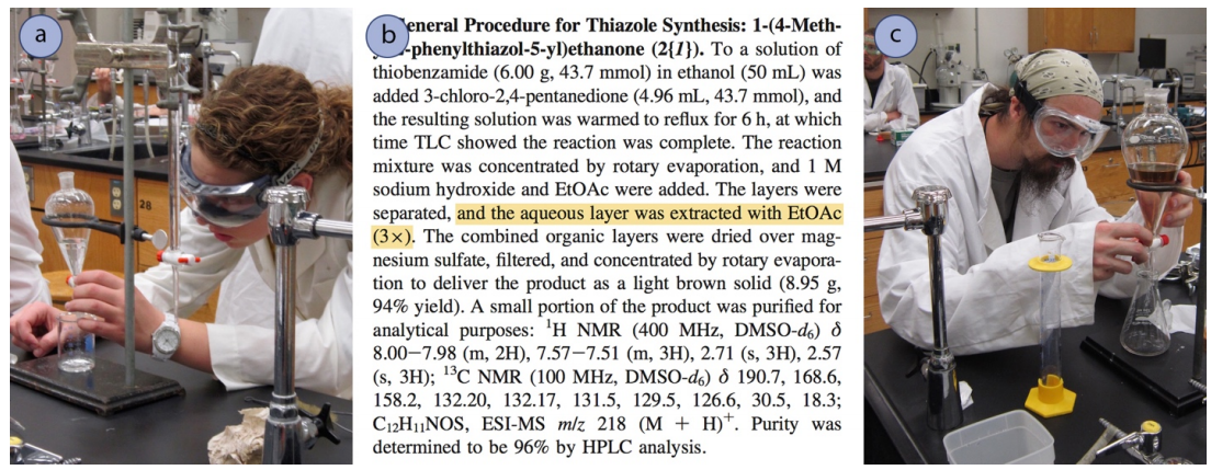
Depending on the partition coefficient for a compound in a solvent, a single extraction may be all that is needed to effectively extract a compound. However, more often than not a procedure calls for a solution to be extracted multiple times to isolate a desired compound, as this method is more efficient than a single extraction (see journal article in Figure 4.15b for an example of where this process is used).

Figure 4.15: a+c) Students using a separatory funnel, b) Journal article from: K. A. Milinkevich, M. J. Kurth, J. Comb. Chem. 2008, 10, 521-525.

In a multiple extraction procedure, a quantity of solvent is used to extract one layer (often the aqueous layer) multiple times in succession. The extraction is repeated two to three times, or perhaps more times if the compound has a low partition coefficient in the organic solvent. Figure 4.16 shows a diagram of an aqueous solution being extracted twice with diethyl ether. Diethyl ether has a density less than \(1 \: \text{g/mL}\), so is the top organic layer in the funnel.

Figure 4.16: Multiple Extractions of an aqueous layer when the organic layer is on the top: a) First extraction, b) Second extraction.

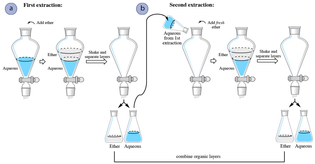
In a multiple extraction of an aqueous layer, the first extraction is procedurally identical to a single extraction. In the second extraction, the aqueous layer from the first extraction is returned to the separatory funnel (Figure 4.16b), with the goal of extracting additional compound. Since the organic layer from the first extraction had already reached equilibrium with the aqueous layer, it would do little good to return it to the separatory funnel and expose it to the aqueous layer again. Instead, fresh diethyl ether is added to the aqueous layer, since it has the potential to extract more compound.

The process is often repeated with a third extraction (not shown in Figure 4.16), with the aqueous layer from the second extraction being returned to the separatory funnel, followed by another portion of fresh organic solvent. In multiple extractions, the organic layers are combined together,as the goal is to extract the compound into the organic solvent.

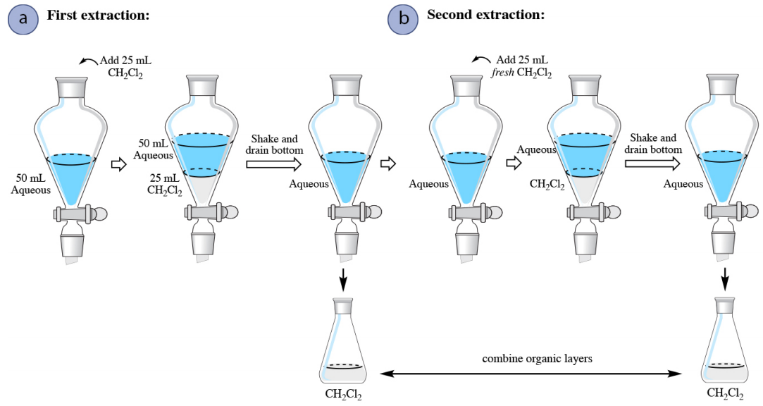
When an aqueous solution is extracted with an organic solvent that is denser than water (for example dichloromethane, \(\ce{CH_2Cl_2}\)), the only procedural difference is that there is no need to ever drain the aqueous layer from the separatory funnel. After draining the organic layer from the first extraction, fresh solvent can be added to the aqueous layer remaining in the funnel to begin the second extraction (Figure 4.17b).

Figure 4.17: Multiple Extractions of an aqueous layer when the organic layer is on the bottom: a) First extraction, b) Second extraction.

\(^2\)The partition coefficients were approximated using solubility data found in: A. Seidell, Solubilities of Inorganic and Organic Substances, D. Van. Nostrand Company, 1907.

\(^3\)From: The Merck Index, 12\(^\text{th}\) edition, Merck Research Laboratories, 1996.