10.3.4: The Fluorescence Lifetime and Quenching

The fluorescence Lifetime is the average time it takes for a molecule after absorption to return to its ground state.  While the fluorescence process for a individual fluorophore is a stochastic process Absorption and emission processes are almost always studied on populations of molecules and the average properties of a molecule of the population are deduced from the macroscopic properties of the process.

In order to describe the behavior of the excited state population we define the following:

• n is the number of molecules in the ground state (•) at time t.

• n * is the number of excited molecules (•) at time t.

• Γ is the rate constant of emission. The dimensions of Γ are sec^-1 (transitions per molecule per unit time).

• f(t) is an arbitrary function of the time, describing the time course of the excitation .

 

In Figure\(\PageIndex{1}\): a laser beam is shown passing through a solution containing fluorophores.  At any given time some fluorophores will be excited (•), while the rest will be in its ground state (•).

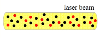
Figure\(\PageIndex{1}\): was taken from Fluorescence Workshop UMN Physics June 8-10, 2006 Fluorescence Lifetime + Polarization (2) presented by Joachim Mueller (https://fitzkee.chemistry.msstate.ed...90/Fluoro5.pdf)

The excited state population of fluorophores is described by a rate equation:

\(\frac{d n^{*}}{d t}=-n^{*} \Gamma+n f(t)\)

where n + n* = n₀ (n₀ describes the total number of molecules and i s a constant)

As shown in Figure\(\PageIndex{2}\): , the excitation intensity in a steady-state experiment is constant. In other words the function f(t) is constant.  The solution of the rate equation for a constant f(t) is given by a constant excited state population:

\(n^{*}=\frac{n_{0} I_{e x}}{\Gamma+I_{e x}}\)

where f(t) = I_ex describes the excitation intensity.  Note that the fluorescence intensity is directly proportional to the excited state population: I_F ∝ n*

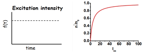
Figure\(\PageIndex{2}\) was taken from Fluorescence Workshop UMN Physics June 8-10, 2006 Fluorescence Lifetime + Polarization (2) presented by Joachim Mueller (https://fitzkee.chemistry.msstate.ed...90/Fluoro5.pdf)

The excited state population is initially directly proportional to the excitation intensity I_ex (linear regime), but saturates at higher excitation intensities (because one can not drive more molecules in the excited state than are available).

In general, steady state experiments are conducted under conditions where we are far from saturation, where n * ∝ I_ex

Lets consider a different experiment, shown in Figure\(\PageIndex{3}\), involving a short pulse of excitation light, much shorter than the lifetime of the fluorophore, say less than 10^-12 s in duration) applied to the sample at t = 0.

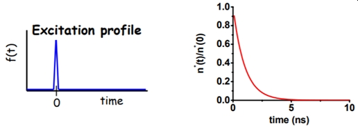
Figure\(\PageIndex{3}\) was taken from Fluorescence Workshop UMN Physics June 8-10, 2006 Fluorescence Lifetime + Polarization (2) presented by Joachim Mueller (https://fitzkee.chemistry.msstate.ed...90/Fluoro5.pdf)

The solution of the rate equation is given by an exponential decay of the excited state population:

\(n^{*}(t)=n^{*}(0) e^{-r t}\)

If a population of fluorophores are excited, the lifetime is the time it takes for the number of excited molecules to decay to 1/e or 36.8% of the original population according to:

\(\frac{n^{*}(t)}{n^{*}(0)}=e^{-t / \tau}\) 

and we can define the lifetime, \({\tau}\) as equal to Γ^-1.

Experimentally we can only observe the radiative (fluorescent) decay. Nonradiative processes are alternative paths for the molecule to return to its ground state. These additional paths lead to a faster decay ( of the excited state population. Thus we observe a faster decay of the fluorescence intensity.

The lifetime and quantum yield for a given fluorophore is often dramatically affected by its environment.  In the gas phase fluorescence lifetimes are the long because there is little interaction with bath molecules leading to non radiative deactivation.  In condensed media the lifetime is a reporter of the local environment of the fluorophore.  For example, NADH, has a lifetime in water of  ~ 0.4 ns but when bound to dehydrogenases the lifetime can be a long as 9 ns.

Commercial instruments for fluorescence lifetime measurements are readily available and based either the impulse response (as described above) or the harmonic response method which relies on a modulated excitation beam and the relative phase lag of the emitted light. In principle both methods have the same information content. These methods are also referred to as either the “time domain” method or the “frequency domain” method and will be left to the curious student to discover and learn about on their own.

Fluorescence Quenching and Fluorescence Resonance Energy Transfer

As said in the section on the Stokes shift, fluorescence is a very sensitive method for studying the local environment around the fluorophore.  Two methods are very commonly employed to learn about the local environment on a molecular scale are  quenching and Fluorescence Resonance Energy Transfer (FRET and not yet discussed in this LibreText).  Quenching can also be employed for quantitative work and the interactions between anions and quenchers is a useful way to measure the concentration of the anions.

Quenching occurs via two distinct pathways. Collisional quenching occurs when the excited state fluorophore is deactivated upon contact with some quencher molecule in solution.  Static quenching occurs when a fluorophore forms a non-fluorescent complex with a quencher and is no longer excitable.

Let's consider the quantum yield for a fluorophore in the absence of a quenching species

\(\phi_{\text {with out quench}}=\frac{k_{f}}{k_{f}+k_{i s c}+k_{i c}}\)

and in the presence of a quencher, Q

\(\phi_{\text {with quench}}=\frac{k_{f}}{k_{f}+k_{i s c}+k_{i c}+k_{\text {quench}}[Q]}\)

the ratio of these two equations yields 

\(\frac{\phi_{\text {vithoutquench }}}{\phi_{\text {withquench }}}=1+\frac{k_{\text {quench}}[Q]}{k_{f}+k_{i s c}+k_{i c}}=1+k_{\text {quench}}[Q]=\mathrm{F}_{0} / \mathrm{F}\)

The expression 

\(\frac{\mathrm{F}_{0}}{\mathrm{F}}=\frac{\tau_{0}}{\tau}=1+K[\mathrm{Q}]\)

is known as the Stern-Volmer equation and the equivalence to the ratio of the fluorescence lifetimes without, 
\({\tau_0}\), and with, \({\tau}\), the quencher only holds for the collisional quencher case.

An experiment done last year in the physical chemistry laboratory was focused on the time scales for the quenching of anthracene's fluorescence by carbon tetrachloride.  In the laboratory portion of this course we will examine the quenching of a sulfonated quinine dye, SPQ by chloride to develop a method for the measurement of the concentration of chloride in solution.

One can often determine  whether or not one is dealing with a collisional quencher or a static quenching by examining the extent of quenching as a function of quencher concentration at at least two temperatures.  Consider Figure\(\PageIndex{4}\) comparing the two forms of quenching. 

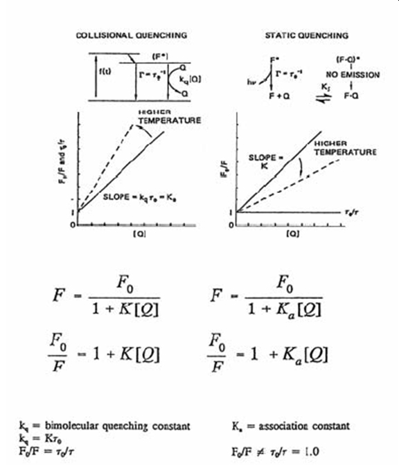
Figure\(\PageIndex{4}\): image source currently unknown

If quenching is occurring by a collisional deactivation of the excited state, according to the kinetic molecular theory, as the temperature of the system is increased the number of collisions between with fluorophore in it's excited state and the quencher will increase and the fluorescence signal will be smaller relative to the the intensity with the same concentration of quencher but at a lower temperature.   Consequently the slope of the Stern-Volmer plot will be greater at the higher temperature relative to the slope at the lower temperature.  The same will be true for a Stern-Volmer plot based on the ratio of the fluorescence lifetimes without, \({\tau_0}\), and with, \({\tau}\), the quencher.

If static quenching is causing the decrease in the fluorscence and increase in system temperature is more likely to rupture the bond associating the fluorophore and quencher resulting in an increase in the fluorescence intensity.  For static quenching the slope of the Stern-Volmer plot will be less at the higher temperature relative to the slope at lower temperature.  Since the observed liftime is only based on the free fluorphores the ratio of of the fluorescence lifetimes without, \({\tau_0}\), and with, \({\tau}\), the quencher will be unchanged.