9.6.2: Chemical Kinetics

The earliest analytical methods based on chemical kinetics—which first appear in the late nineteenth century—took advantage of the catalytic activity of enzymes. In a typical method of that era, an enzyme was added to a solution that contained a suitable substrate and their reaction was monitored for a fixed time. The enzyme’s activity was determined by the change in the substrate’s concentration. Enzymes also were used for the quantitative analysis of hydrogen peroxide and carbohydrates. The development of chemical kinetic methods continued in the first half of the twentieth century with the introduction of nonenzymatic catalysts and noncatalytic reactions.

Despite the diversity of chemical kinetic methods, by 1960 they no longer were in common use. The principal limitation to their broader acceptance was a susceptibility to significant errors from uncontrolled or poorly controlled variables—temperature and pH are two such examples—and the presence of interferents that activate or inhibit catalytic reactions. By the 1980s, improvements in instrumentation and data analysis methods compensated for these limitations, ensuring the further development of chemical kinetic methods of analysis [Pardue, H. L. Anal. Chim. Acta 1989, 216, 69–107].

Theory and Practice

Every chemical reaction occurs at a finite rate, which makes it a potential candidate for a chemical kinetic method of analysis. To be effective, however, the chemical reaction must meet three necessary conditions: (1) the reaction must not occur too quickly or too slowly; (2) we must know the reaction’s rate law; and (3) we must be able to monitor the change in concentration for at least one species. Let’s take a closer look at each of these requirements.

The material in this section assumes some familiarity with chemical kinetics, which is part of most courses in general chemistry. For a review of reaction rates, rate laws, and integrated rate laws, see the material in Appendix 17.

Reaction Rate

The rate of the chemical reaction—how quickly the concentrations of reactants and products change during the reaction—must be fast enough that we can complete the analysis in a reasonable time, but also slow enough that the reaction does not reach equilibrium while the reagents are mixing. As a practical limit, it is not easy to study a reaction that reaches equilibrium within several seconds without the aid of special equipment for rapidly mixing the reactants.

We will consider two examples of instrumentation for studying reactions with fast kinetics later in this chapter.

Rate Law

The second requirement is that we must know the reaction’s rate law—the mathematical equation that describes how the concentrations of reagents affect the rate—for the period in which we are making measurements. For example, the rate law for a reaction that is first order in the concentration of an analyte, A, is

\[\text { rate }=-\frac{d[A]}{d t}=k[A] \label{13.1}\]

where k is the reaction’s rate constant.

Because the concentration of A decreases during the reactions, d[A] is negative. The minus sign in equation \ref{13.1} makes the rate positive. If we choose to follow a product, P, then d[P] is positive because the product’s concentration increases throughout the reaction. In this case we omit the minus sign.

An integrated rate law often is a more useful form of the rate law because it is a function of the analyte’s initial concentration. For example, the integrated rate law for equation \ref{13.1} is

\[\ln{[A]_t} = \ln{[A]_0} - kt \label{13.2}\]

or

\[[A]_{t}=[A]_{0} e^{-k t} \label{13.3}\]

where [A]₀ is the analyte’s initial concentration and [A]_t is the analyte’s concentration at time t.

Unfortunately, most reactions of analytical interest do not follow a simple rate law. Consider, for example, the following reaction between an analyte, A, and a reagent, R, to form a single product, P

\[A + R \rightleftharpoons P \nonumber\]

where k_f is the rate constant for the forward reaction, and k_r is the rate constant for the reverse reaction. If the forward and the reverse reactions occur as single steps, then the rate law is

\[\text { rate }=-\frac{d[A]}{d t}=k_{f}[A][R]-k_{r}[P] \label{13.4}\]

The first term, k_f[A][R] accounts for the loss of A as it reacts with R to make P, and the second term, k_r[P] accounts for the formation of A as P converts back to A and to R.

Although we know the reaction’s rate law, there is no simple integrated form that we can use to determine the analyte’s initial concentration. We can simplify equation \ref{13.4} by restricting our measurements to the beginning of the reaction when the concentration of product is negligible.

Under these conditions we can ignore the second term in equation \ref{13.4}, which simplifies to

\[\text { rate }=-\frac{d[A]}{d t}=k_{f}[A][R] \label{13.5}\]

The integrated rate law for equation \ref{13.5}, however, is still too complicated to be analytically useful. We can further simplify the kinetics by making further adjustments to the reaction conditions [Mottola, H. A. Anal. Chim. Acta 1993, 280, 279–287]. For example, we can ensure pseudo-first-order kinetics by using a large excess of R so that its concentration remains essentially constant during the time we monitor the reaction. Under these conditions equation \ref{13.5} simplifies to

\[\text { rate }=-\frac{d[A]}{d t}=k_{f}[A][R]_{0}=k^{\prime}[A] \label{13.6}\]

where k′ = k_f[R]₀. The integrated rate law for equation \ref{13.6} then is

\[\ln{[A]_t} = \ln{[A]_0} - k’t \label{13.7}\]

or

\[[A]_{t}=[A]_{0} e^{-k^{\prime} t} \label{13.8}\]

It may even be possible to adjust the conditions so that we use the reaction under pseudo-zero-order conditions.

\[\text { rate }=-\frac{d[A]}{d t}=k_{f}[A]_{0}[R]_{0}=k^{\prime \prime} t \label{13.9}\]

\[[A]_{t}=[A]_{0}-k^{\prime \prime} t \label{13.10}\]

where \(k^{\prime \prime}\) = k_f [A]₀[R]₀.

To say that the reaction is pseudo-first-order in A means the reaction behaves as if it is first order in A and zero order in R even though the underlying kinetics are more complicated. We call \(k^{\prime}\) a pseudo-first-order rate constant. To say that a reaction is pseudo-zero-order means the reaction behaves as if it is zero order in A and zero order in R even though the underlying kinetics are more complicated. We call \(k^{\prime \prime}\) the pseudo-zero-order rate constant.

Monitoring the Reaction

The final requirement is that we must be able to monitor the reaction’s progress by following the change in concentration for at least one of its species. Which species we choose to monitor is not important: it can be the analyte, a reagent that reacts with the analyte, or a product. For example, we can determine the concentration of phosphate by first reacting it with Mo(VI) to form 12-molybdophosphoric acid (12-MPA).

\[\mathrm{H}_{3} \mathrm{PO}_{4}(a q)+6 \mathrm{Mo}(\mathrm{VI})(a q) \longrightarrow 12-\mathrm{MPA}(a q)+9 \mathrm{H}^{+}(a q) \label{13.11}\]

Next, we reduce 12-MPA to heteropolyphosphomolybdenum blue, PMB. The rate of formation of PMB is measured spectrophotometrically, and is proportional to the concentration of 12-MPA. The concentration of 12-MPA, in turn, is proportional to the concentration of phosphate [see, for example, (a) Crouch, S. R.; Malmstadt, H. V. Anal. Chem. 1967, 39, 1084–1089; (b) Crouch, S. R.; Malmstadt, H. V. Anal. Chem. 1967, 39, 1090–1093; (c) Malmstadt, H. V.; Cordos, E. A.; Delaney, C. J. Anal. Chem. 1972, 44(12), 26A–41A]. We also can follow reaction 13.11 spectrophotometrically by monitoring the formation of the yellow-colored 12-MPA [Javier, A. C.; Crouch, S. R.; Malmstadt, H. V. Anal. Chem. 1969, 41, 239–243].

Reaction \ref{13.11} is, of course, unbalanced; the additional hydrogens on the reaction’s right side come from the six Mo(VI) that appear on the reaction’s left side where Mo(VI) is thought to be present as the molybdate dimer HMo₂O₆⁺.

There are several advantages to using the reaction’s initial rate (t = 0). First, because the reaction’s rate decreases over time, the initial rate provides the greatest sensitivity. Second, because the initial rate is measured under nearly pseudo-zero-order conditions, in which the change in concentration with time effectively is linear, it is easier to determine the slope. Finally, as the reaction of interest progresses competing reactions may develop, which complicating the kinetics: using the initial rate eliminates these complications. One disadvantage of the initial rate method is that there may be insufficient time to completely mix the reactants. This problem is avoided by using an intermediate rate measured at a later time (t > 0).

As a general rule (see Mottola, H. A. “Kinetic Determinations of Reactants Utilizing Uncatalyzed Reactions,” Anal. Chim. Acta 1993, 280, 279–287), the time for measuring a reaction’s initial rate should result in the consumption of no more than 2% of the reactants. The smaller this percentage, the more linear the change in concentration as a function of time.

 

 

Representative Method 13.2.1: Determination of Creatinine in Urine

Description of Method

Creatine is an organic acid in muscle tissue that supplies energy for muscle contractions. One of its metabolic products is creatinine, which is excreted in urine. Because the concentration of creatinine in urine and serum is an important indication of renal function, a rapid method for its analysis is clinically important. In this method the rate of reaction between creatinine and picrate in an alkaline medium is used to determine the concentration of creatinine in urine. Under the conditions of the analysis the reaction is first order in picrate, creatinine, and hydroxide.

\[\text { rate }=k[\text { picrate }][\text { creatinine }]\left[\mathrm{OH}^{-}\right] \nonumber\]

The reaction is monitored using a picrate ion selective electrode.

Procedure

Prepare a set of external standards that contain 0.5–3.0 g/L creatinine using a stock solution of 10.00 g/L creatinine in 5 mM H₂SO₄, diluting each standard to volume using 5 mM H₂SO₄. Prepare a solution of \(1.00 \times 10^{-2}\) M sodium picrate. Pipet 25.00 mL of 0.20 M NaOH, adjusted to an ionic strength of 1.00 M using Na₂SO₄, into a thermostated reaction cell at 25^oC. Add 0.500 mL of the \(1.00 \times 10^{-2}\) M picrate solution to the reaction cell. Suspend a picrate ion selective in the solution and monitor the potential until it stabilizes. When the potential is stable, add 2.00 mL of a creatinine external standard and record the potential as a function of time. Repeat this procedure using the remaining external standards. Construct a calibration curve of \(\Delta E / \Delta t\) versus the initial concentration of creatinine. Use the same procedure to analyze samples, using 2.00 mL of urine in place of the external standard. Determine the concentration of creatinine in the sample using the calibration curve.

Questions

1. The analysis is carried out under conditions that are pseudo-first order in picrate. Show that under these conditions the change in potential as a function of time is linear.

The potential, E, of the picrate ion selective electrode is given by the Nernst equation

\[E=K-\frac{R T}{F} \ln{[\text { picrate }]} \nonumber\]

where K is a constant that accounts for the reference electrodes, the junction potentials, and the ion selective electrode’s asymmetry potential, R is the gas constant, T is the temperature, and F is Faraday’s constant. We know from equation \ref{13.7} that for a pseudo-first-order reaction, the concentration of picrate at time t is

\[\ln {[\text{picrate}]_t}=\ln{[\text {picrate}]}_{0}-k^{\prime} t \nonumber\]

where \(k^{\prime}\) is the pseudo-first-order rate constant. Substituting this integrated rate law into the ion selective electrode’s Nernst equation leaves us with the following result.

\[E_{t} = K - \frac{R T} {F} \left( \ln{[\text {picrate}]}_{0} - k^{\prime} t\right) \nonumber\]

\[E_{t} = K - \frac{R T} {F} \ln{[\text {picrate}]}_{0} + \frac{R T} {F} k^{\prime}t \nonumber\]

Because K and (RT/F)ln[picrate]₀ are constants, a plot of E_t versus t is a straight line with a slope of \(\frac{R T} {F} k^{\prime}\).

2. Under the conditions of the analysis, the rate of the reaction is pseudo-first-order in picrate and pseudo-zero-order in creatinine and OH^–. Explain why it is possible to prepare a calibration curve of \(\Delta E / \Delta t\) versus the concentration of creatinine.

The slope of a plot of E_t versus t is \(\Delta E / \Delta t = RTk^{\prime}/F\) = RTk′/F (see the previous question). Because the reaction is carried out under conditions where it is pseudo-zero-order in creatinine and OH^–, the rate law is

\[\text{rate} = k[\text{picrate}][\text{creatinine}]_0[\text{OH}^-]_0 = k^{\prime}[\text{picrate}] \nonumber\]

The pseudo-first-order rate constant, \(k^{\prime}\), is

\[k^{\prime}=k[\text { creatinine }]_{0}\left[\mathrm{OH}^{-}\right]_{0}=c[\text {creatinine}]_{0} \nonumber\]

where c is a constant equivalent to k[OH^-]₀ . The slope of a plot of E_t versus t, therefore, is linear function of creatinine’s initial concentration

\[\frac{\Delta E}{\Delta t}=\frac{R T k^{\prime}}{F}=\frac{R T c}{F}[\text {creatinine}]_{0} \nonumber\]

and a plot of \(\Delta E / \Delta t\) versus the concentration of creatinine can serve as a calibration curve.

3. Why is it necessary to thermostat the reaction cell?

The rate of a reaction is temperature-dependent. The reaction cell is thermostated to maintain a constant temperature to prevent a determinate error from a systematic change in temperature, and to minimize indeterminate errors from random fluctuations in temperature.

4. Why is it necessary to prepare the NaOH solution so that it has an ionic strength of 1.00 M?

The potential of the picrate ion selective electrode actually responds to the activity of the picrate anion in solution. By adjusting the NaOH solution to a high ionic strength we maintain a constant ionic strength in all standards and samples. Because the relationship between activity and concentration is a function of ionic strength, the use of a constant ionic strength allows us to write the Nernst equation in terms of picrate’s concentration instead of its activity.

Making Kinetic Measurements

When using Representative Method 13.2.1 to determine the concentration of creatinine in urine, we follow the reactions kinetics using an ion selective electrode. In principle, we can use any of the analytical techniques in Chapters 8–12 to follow a reaction’s kinetics provided that the reaction does not proceed to an appreciable extent during the time it takes to make a measurement. As you might expect, this requirement places a serious limitation on kinetic methods of analysis. If the reaction’s kinetics are slow relative to the analysis time, then we can make a measurement without the analyte undergoing a significant change in concentration. If the reaction’s rate is too fast—which often is the case—then we introduce a significant error if our analysis time is too long.

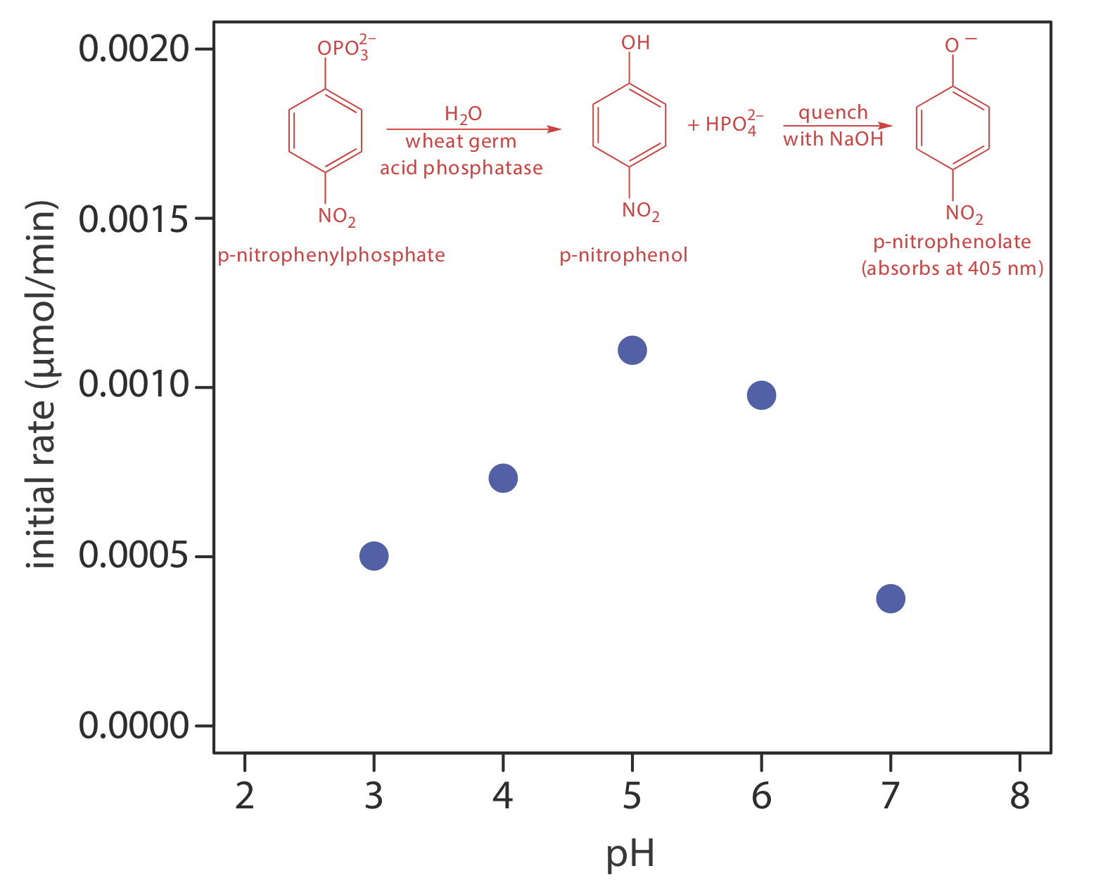
One solution to this problem is to stop, or quench the reaction by adjusting experimental conditions. For example, many reactions show a strong dependence on pH and are quenched by adding a strong acid or a strong base. Figure \(\PageIndex{6}\) shows a typical example for the enzymatic analysis of p-nitrophenylphosphate, which uses the enzyme wheat germ acid phosphatase to hydrolyze the analyte to p-nitrophenol. The reaction has a maximum rate at a pH of 5. Increasing the pH by adding NaOH quenches the reaction and converts the colorless p-nitrophenol to the yellow-colored p-nitrophenolate, which absorbs at 405 nm.

Figure \(\PageIndex{6}\). Initial rate for the enzymatic hydrolysis of p-nitrophenylphosphate using wheat germ acid phosphatase. Increasing the pH quenches the reaction and coverts colorless p-nitrophenol to the yellow-colored p-nitrophenolate, which absorbs at 405 nm.

An additional problem when the reaction’s kinetics are fast is ensuring that we rapidly and reproducibly mix the sample and the reagents. For a fast reaction, we need to make our measurements within a few seconds—or even a few milliseconds—of combining the sample and reagents. This presents us with a problem and an advantage. The problem is that rapidly and reproducibly mixing the sample and the reagent requires a dedicated instrument, which adds an additional expense to the analysis. The advantage is that a rapid, automated analysis allows for a high throughput of samples. Instruments for the automated kinetic analysis of phosphate using reaction \ref{13.11}, for example, have sampling rates of approximately 3000 determinations per hour.

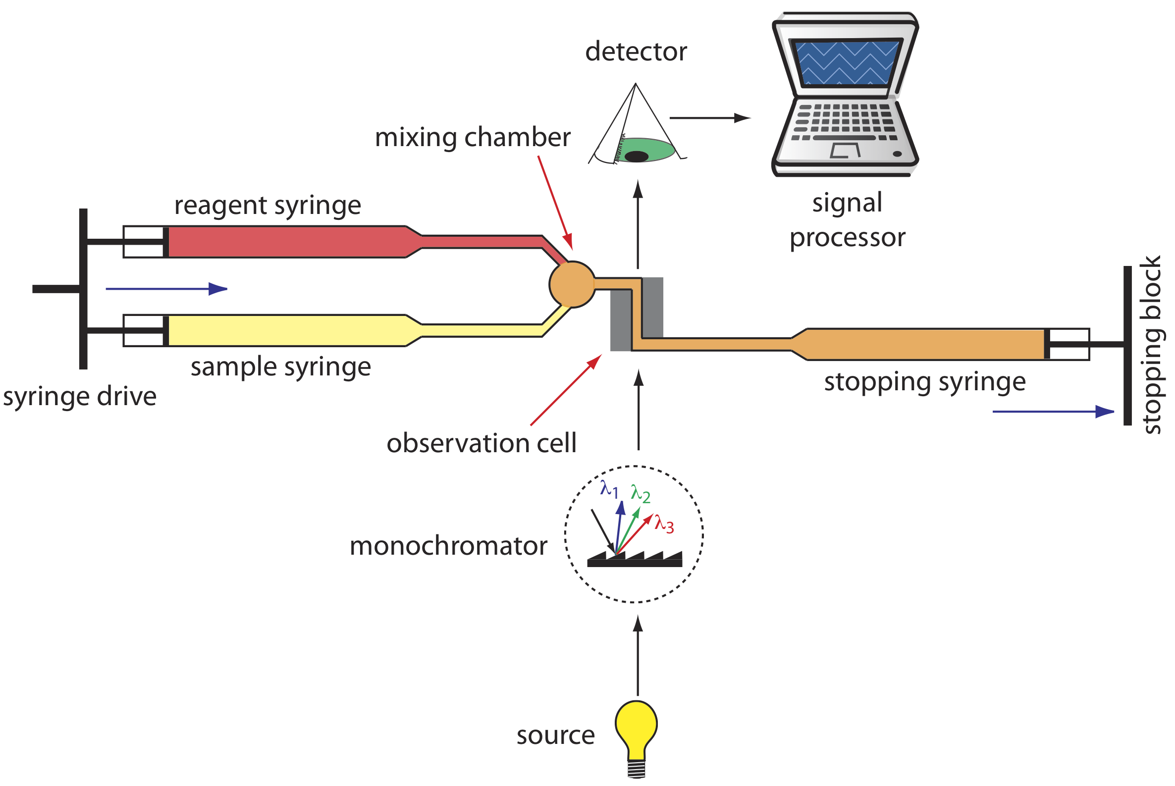
A variety of instruments have been developed to automate the kinetic analysis of fast reactions. One example, which is shown in Figure \(\PageIndex{7}\), is the stopped-flow analyzer. The sample and the reagents are loaded into separate syringes and precisely measured volumes are dispensed into a mixing chamber by the action of a syringe drive. The continued action of the syringe drive pushes the mixture through an observation cell and into a stopping syringe. The back pressure generated when the stopping syringe hits the stopping block completes the mixing, after which the reaction’s progress is monitored spectrophotometrically. With a stopped-flow analyzer it is possible to complete the mixing of sample and reagent, and initiate the kinetic measurements in approximately 0.5 ms. By attaching an autosampler to the sample syringe it is possible to analyze up to several hundred samples per hour.

Figure \(\PageIndex{7}\). Schematic diagram of a stopped-flow analyzer. The blue arrows show the direction in which the syringes are moving.

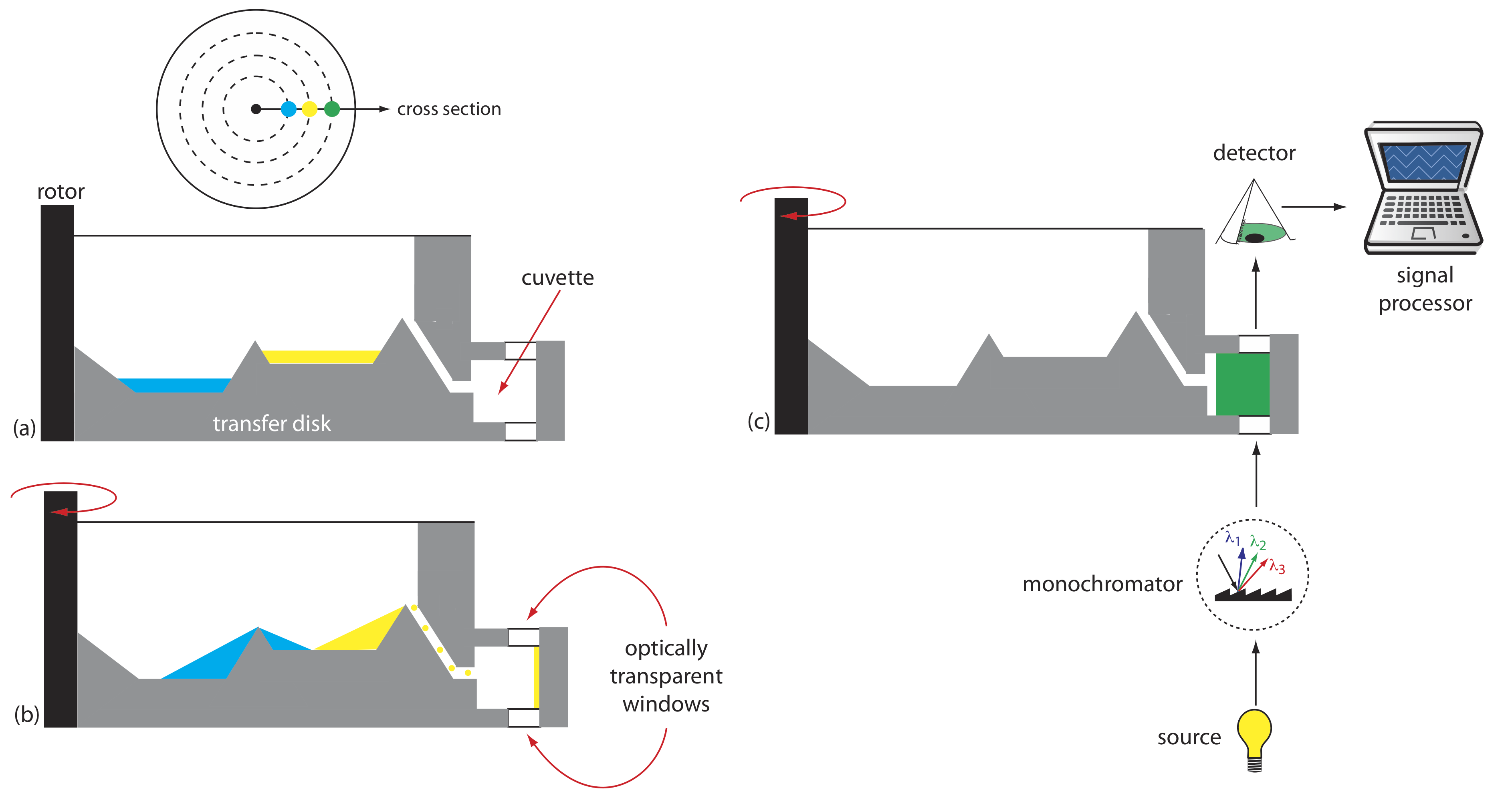
Another instrument for kinetic measurements is the centrifugal analyzer, a partial cross section of which is shown in Figure \(\PageIndex{8}\). The sample and the reagents are placed in separate wells, which are oriented radially around a circular transfer disk. As the centrifuge spins, the centrifugal force pulls the sample and the reagents into the cuvette where mixing occurs. A single optical source and detector, located below and above the transfer disk’s outer edge, measures the absorbance each time the cuvette passes through the optical beam. When using a transfer disk with 30 cuvettes and rotating at 600 rpm, we can collect 10 data points per second for each sample.

Figure \(\PageIndex{8}\). Cross sections through a centrifugal analyzer showing (a) the wells that hold the sample and the reagents, (b) the mixing of the sample and the reagents, and (c) the configuration of the spectrophotometric detector.

The ability to collect lots of data and to collect it quickly requires appropriate hardware and software. Not surprisingly, automated kinetic analyzers developed in parallel with advances in analog and digital circuitry—the hardware—and computer software for smoothing, integrating, and differentiating the analytical signal. For an early discussion of the importance of hardware and software, see Malmstadt, H. V.; Delaney, C. J.; Cordos, E. A. “Instruments for Rate Determinations,” Anal. Chem. 1972, 44(12), 79A–89A.