9.2: The Equations of Enzyme Kinetics

In biological systems, enzymes act as catalysts and play a critical role in accelerating reactions, anywhere from $10^3$ to $10^{17}$ times faster than the reaction would normally proceed. Enzymes are high-molecular weight proteins that act on a substrate, or reactant molecule, to form one or more products.

Michaelis-Menten Enzyme Kinetics

Enzymes are highly specific catalysts for biochemical reactions, with each enzyme showing a selectivity for a single reactant, or substrate. For example, the enzyme acetylcholinesterase catalyzes the decomposition of the neurotransmitter acetylcholine to choline and acetic acid. Many enzyme–substrate reactions follow a simple mechanism that consists of the initial formation of an enzyme–substrate complex, $ES$, which subsequently decomposes to form product, releasing the enzyme to react again.

Figure $\PageIndex{1}$: An enzyme catalyzes the reaction of two substrates and to form one product. from Wikipedia.

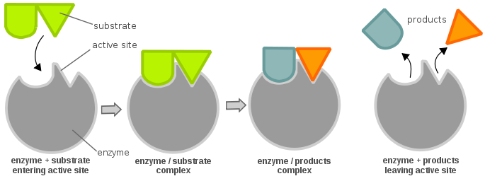
This is described within the following multi-step mechanism

$$E + S \underset{k_{-1}}{\overset{k_1}{\rightleftharpoons}} ES \underset{k_{-2}}{\overset{k_2}{\rightleftharpoons}} E + P \label{13.20}$$

where $k_1$, $k_{–1}$, $k_2$, and $k_{–2}$ are rate constants. The reaction’s rate law for generating the product $[P]$ is

$$rate = \dfrac{d[P]}{dt} = k_2[ES] - k_{-2}[E][P] \label{13.21A}$$

However, if we make measurement early in the reaction, the concentration of products is negligible, i.e.,

$$[P] \approx 0$$

and we can ignore the back reaction (second term in right side of Equation $\ref{13.21A}$). Then under these conditions, the reaction’s rate is

$$rate = \dfrac{d[P]}{dt} = k_2[ES] \label{13.21}$$

To be analytically useful we need to write Equation $\ref{13.21}$ in terms of the reactants (e.g., the concentrations of enzyme and substrate). To do this we use the steady-state approximation, in which we assume that the concentration of $ES$ remains essentially constant. Following an initial period, during which the enzyme–substrate complex first forms, the rate at which $ES$ forms

$$\dfrac{d[ES]}{dt} =k_1[E] [S] = k_1([E]_0 − [ES])[S] \label{13.22}$$

is equal to the rate at which it disappears

$$− \dfrac{d[ES]}{dt} = k_{−1}[ES] + k_2[ES] \label{13.23}$$

where $[E]_0$ is the enzyme’s original concentration. Combining Equations $\ref{13.22}$ and $\ref{13.23}$ gives

$$k_1([E]_0 − [ES]) [S] = k_{−1}[ES] + k_2[ES]$$

which we solve for the concentration of the enzyme–substrate complex

$$[ES] = \dfrac{ [E]_0[S] }{ \dfrac{k_{−1} + k_2}{k_1} + [S] } = \dfrac{[E]_0[S] }{K_m + [S]} \label{Eq13.24}$$

where $K_m$ is the Michaelis constant. Substituting Equation $\ref{Eq13.24}$ into Equation $\ref{13.21}$ leaves us with our final rate equation.

$$\dfrac{d[P]}{dt} = \dfrac{k_2[E]_0[S]}{K_m + [S]} \label{Eq13.25}$$

A plot of Equation $\ref{Eq13.25}$, as shown in Figure $\PageIndex{1}$, is instructive for defining conditions where we can use the rate of an enzymatic reaction for the quantitative analysis of an enzyme or substrate.

Figure $\PageIndex{1}$: Plot of Equation $\ref{Eq13.25}$ showing limits for the analysis of substrates and enzymes in an enzyme-catalyzed chemical kinetic method of analysis. The curve in the region highlighted in red obeys equation $\ref{13.27}$ and the curve in the area highlighted in green follows Equation $\ref{Eq13.26}$.

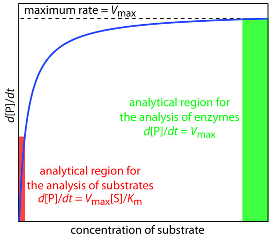
For high substrate concentrations, where $[S] \gg K_m$, Equation $\ref{Eq13.25}$ simplifies to

$$\dfrac{d[P]}{dt} = \dfrac{k_2[E]_0[S]}{ K_m + [S]} \approx \dfrac{k_2[E]_0[S]}{[S]} = k_2[E]_0 = V_{max} \label{Eq13.26}$$

where $V_{max}$ is the maximum rate for the catalyzed reaction. Under these conditions the reaction is zero-order in substrate and we can use $V_{max}$ to calculate the enzyme’s concentration, typically using a variable-time method. At lower substrate concentrations, where $[S] \ll K_m$, Equation $\ref{Eq13.25}$ becomes

$$\dfrac{d[P]}{dt} = \dfrac{k_2[E]_0[S]}{K_m + [S]} \approx \dfrac{k_2[E]_0[S]}{ K_m} =\dfrac{V_{max}[S]}{K_m} \label{13.27}$$

The reaction is now first-order in substrate, and we can use the rate of the reaction to determine the substrate’s concentration by a fixed-time method.

The Michaelis constant $K_m$ is the substrate concentration at which the reaction rate is at half-maximum, and is an inverse measure of the substrate's affinity for the enzyme—as a small $K_m$ indicates high affinity, meaning that the rate will approach $V_{max}$ more quickly. The value of $K_m$ is dependent on both the enzyme and the substrate, as well as conditions such as temperature and pH.

The Michaelis constant $K_m$ is the substrate concentration at which the reaction rate is at half-maximum.

From the last two terms in Equation $\ref{13.27}$, we can express $V_{max}$ in terms of a turnover number ($k_{cat}$):

$$V_{max} = k_{cat}[E]_o$$

where $[E]_0$ is the enzyme concentration and $k_{cat}$ is the turnover number, defined as the maximum number of substrate molecules converted to product per enzyme molecule per second. Hence, the turnover number is defined as the maximum number of chemical conversions of substrate molecules per second that a single catalytic site will execute for a given enzyme concentration $[E]_o$.

Example $\PageIndex{1}$: Turnover number of acetylcholinesterase

Acetylcholinesterase (AChE) may be one of the fastest enzymes. It hydrolyzes acetylcholine to choline and an acetate group. One of the earliest values of the turnover number was $3 \times 10^7$ (molecules of acetylcholine) per minute per molecule of enzyme. A more recent value at 25°C, pH = 7.0, acetylcholine concentration of $2.5 \times 10^{−3}\; M$, was found to be $7.4 \times 10^5\; min^{−1}$ (J Biol Chem. 236 (8): 2292–5.).

There may be some 30 active centers per molecule. AChE is a serine hydrolase that reacts with acetylcholine at close to the diffusion-controlled rate. A diffusion-controlled reaction occurs so quickly that the reaction rate is the rate of transport of the reactants through the solution; as quickly as the reactants encounter each other, they react.

The Significance of $K_M$ and $V_{max}$

The Michaelis-Menten model is used in a variety of biochemical situations other than enzyme-substrate interaction, including antigen-antibody binding, DNA-DNA hybridization, and protein-protein interaction. It can be used to characterize a generic biochemical reaction, in the same way that the Langmuir equation can be used to model generic adsorption of biomolecular species. When an empirical equation of this form is applied to microbial growth. The experimentally determined parameters values vary wildly between enzymes (Table $\PageIndex{1}$):

Table $\PageIndex{1}$: Enzyme Kinetic parameters

Enzyme	$K_m$ (M)	$k_{cat}$ (1/s)	$k_{cat}/K_m$ (1/M.s)
Chymotrypsin	1.5 × 10^−2	0.14	9.3
Pepsin	3.0 × 10^−4	0.50	1.7 × 10^3
Tyrosyl-tRNA synthetase	9.0 × 10^−4	7.6	8.4 × 10^3
Ribonuclease	7.9 × 10^−3	7.9 × 10^2	1.0 × 10^5
Carbonic anhydrase	2.6 × 10^−2	4.0 × 10^5	1.5 × 10^7
Fumarase	5.0 × 10^−6	8.0 × 10^2	1.6 × 10^8

While $K_m$ is equal to the substrate concentration at which the enzyme converts substrates into products at half its maximal rate and hence is related to the affinity of the substrate for the enzyme. The catalytic rate $k_{cat}$ is the rate of product formation when the enzyme is saturated with substrate and therefore reflects the enzyme's maximum rate. The rate of product formation is dependent on both how well the enzyme binds substrate and how fast the enzyme converts substrate into product once substrate is bound. For a kinetically perfect enzyme, every encounter between enzyme and substrate leads to product and hence the reaction velocity is only limited by the rate the enzyme encounters substrate in solution. From Equation $\ref{Eq13.24}$, the catalytic efficiency of a protein can be evaluated.

$$\dfrac{k_{cat}}{K_m} = \dfrac{k_2}{K_m} = \dfrac{k_1k_2}{k_{-1} + k_2}$$

This $k_{cat}/K_m$ ratio is called the specificity constant measure of how efficiently an enzyme converts a substrate into product. It has a theoretical upper limit of 10⁸ – 10¹⁰ /M.s; enzymes working close to this, such as fumarase, are termed superefficient (Table $\PageIndex{1}$).

Determining $V_m$ and $K_m$ from experimental data can be difficult and the most common way is to determine initial rates, $v_0$, from experimental values of $[P]$ or $[S]$ as a function of time. Hyperbolic graphs of $v_0$ vs. $[S]$ can be fit or transformed as we explored with the different mathematical transformations of the hyperbolic binding equation to determine $K_d$. These included:

• nonlinear hyperbolic fit (e.g., Figure $\PageIndex{1}$)
• double reciprocal plot (e.g., Lineweaver–Burk plot discussed below
• Eadie-Hofstee plot

Lineweaver–Burk plot

Another commonly-used plot in examining enzyme kinetics is the Lineweaver-Burk plot, in with the inverse of the reaction rate, $1/r$, is plotted against the inverse of the substrate concentration $1/\left[ \text{S} \right]$. Rearranging Equation $\ref{Eq13.26}$,

$$\dfrac{1}{r} = \dfrac{K_M + \left[ \text{S} \right]}{k_2 \left[ \text{E} \right]_0 \left[ \text{S} \right]} = \dfrac{K_M}{k_2 \left[ \text{E} \right]_0} \dfrac{1}{\left[ \text{S} \right]} + \dfrac{1}{k_2 \left[ \text{E} \right]_0} \label{Eq28}$$

Tthe Lineweaver–Burk plot (or double reciprocal plot) is a graphical representation of the Lineweaver–Burk equation of enzyme kinetics, described by Hans Lineweaver and Dean Burk in 1934 (Figure $\PageIndex{2}$). The Lineweaver-Burk plot results in a straight line with the slope equal to $K_M/k_2 \left[ \text{E} \right]_0$ and $y$-intercept equal to $1/k_2 \left[ \text{E} \right]_0$ which is $1/V_{max}$ via Equation $\ref{Eq13.26}$.

Figure $\PageIndex{2}$: Lineweaver–Burk plot of Michaelis–Menten kineitcs.

The plot provides a useful graphical method for analysis of the Michaelis–Menten equation:

$$V = \dfrac{V_{\max} [S]}{K_m + [S]}$$

Taking the reciprocal gives

$$\dfrac{1}{V} = \dfrac {K_m + [S]} {V_{max}[S]} = \dfrac{K_m}{V_{max}} \dfrac{1}{[S]} + \dfrac{1}{V_{max}}$$

where

• $V$ is the reaction velocity (the reaction rate),
• $K_m$ is the Michaelis–Menten constant,
• $V_{max}$ is the maximum reaction velocity, and
• $[S]$ is the substrate concentration.

The Lineweaver–Burk plot was widely used to determine important terms in enzyme kinetics, such as $K_m$ and $V_{max}$, before the wide availability of powerful computers and non-linear regression software. The y-intercept of such a graph is equivalent to the inverse of $V_{max}$; the x-intercept of the graph represents $−1/K_m$. It also gives a quick, visual impression of the different forms of enzyme inhibition.

Example $\PageIndex{2}$

The reaction between nicotineamide mononucleotide and ATP to form nicotineamide–adenine dinucleotide and pyrophosphate is catalyzed by the enzyme nicotinamide mononucleotide adenylyltransferase. The following table provides typical data obtained at a pH of 4.95. The substrate, S, is nicotinamide mononucleotide and the initial rate, v, is the μmol of nicotinamide–adenine dinucleotide formed in a 3-min reaction period.

[S] (mM)	v (μmol)	[S] (mM)	v (μmol)
0.138	0.148	0.560	0.324
0.220	0.171	0.766	0.390
0.291	0.234	1.460	0.493

Determine values for V_max and K_m.

Solution

Figure 13.12 shows the Lineweaver–Burk plot for this data and the resulting regression equation. Using the y-intercept, we calculate V_max as

V_max= 1 / y−intercept = 1 / 1.708 mol = 0.585 mol

and using the slope we find that K_m is

K_m = slope × V_max = 0.7528 molimM × 0.585 mol = 0.440 mM

Figure 13.12: Linweaver–Burk plot and regression equation for the data in Example 13.6.

Exercise $\PageIndex{2}$: o-diphenyl oxidase

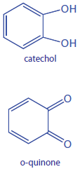
The following data are for the oxidation of catechol (the substrate) to o-quinone by the enzyme o-diphenyl oxidase. The reaction is followed by monitoring the change in absorbance at 540 nm. The data in this exercise are adapted from jkimball.

[catechol] (mM)	0.3	0.6	1.2	4.8
rate (∆AU/min)	0.020	0.035	0.048	0.081

Determine values for V_max and K_m.

Click here to review your answer to this exercise.

The double reciprocal plot distorts the error structure of the data, and it is therefore unreliable for the determination of enzyme kinetic parameters. Although it is still used for representation of kinetic data, non-linear regression or alternative linear forms of the Michaelis–Menten equation such as the Hanes-Woolf plot or Eadie–Hofstee plot are generally used for the calculation of parameters.

Problems with the Method

The Lineweaver–Burk plot is classically used in older texts, but is prone to error, as the y-axis takes the reciprocal of the rate of reaction – in turn increasing any small errors in measurement. Also, most points on the plot are found far to the right of the y-axis (due to limiting solubility not allowing for large values of $[S]$ and hence no small values for $1/[S]$), calling for a large extrapolation back to obtain x- and y-intercepts^.

When used for determining the type of enzyme inhibition, the Lineweaver–Burk plot can distinguish competitive, non-competitive and uncompetitive inhibitors. Competitive inhibitors have the same y-intercept as uninhibited enzyme (since $V_{max}$ is unaffected by competitive inhibitors the inverse of $V_{max}$ also doesn't change) but there are different slopes and x-intercepts between the two data sets. Non-competitive inhibition produces plots with the same x-intercept as uninhibited enzyme ($K_m$ is unaffected) but different slopes and y-intercepts. Uncompetitive inhibition causes different intercepts on both the y- and x-axes but the same slope.

Eadie–Hofstee Plot

The Eadie–Hofstee plot is a graphical representation of enzyme kinetics in which reaction rate is plotted as a function of the ratio between rate and substrate concentration and can be derived from the Michaelis–Menten equation ($\ref{Eq13.25}$) by inverting and multiplying with $V_{max}$:

$$\dfrac{V_{max}}{v} = \dfrac{V_{max}(K_m+[S])}{V_{max}[S]} = \dfrac{K_m+[S]}{[S]}$$

Rearrange:

$$V_{max} = \dfrac{vK_m}{[S]} + \dfrac{v[S]}{[S]} = \dfrac{v K_m}{[S]} + v$$

Isolate v:

$$v = -K_m \dfrac{v}{[S]} + V_{max}$$

Figure $\PageIndex{3}$: The Eadie-Hofstee plot is a more accurate linear plotting method with v is plotted against v/[S].

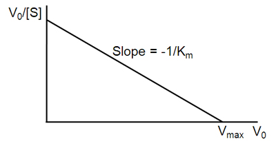
A plot of v against $v/[S]$ will hence yield $V_{max}$ as the y-intercept, $V_{max}/K_m$ as the x-intercept, and $K_m$ as the negative slope (Figure $\PageIndex{3}$). Like other techniques that linearize the Michaelis–Menten equation, the Eadie-Hofstee plot was used historically for rapid identification of important kinetic terms like $K_m$ and $V_{max}$, but has been superseded by nonlinear regression methods that are significantly more accurate and no longer computationally inaccessible. It is also more robust against error-prone data than the Lineweaver–Burk plot, particularly because it gives equal weight to data points in any range of substrate concentration or reaction rate (the Lineweaver–Burk plot unevenly weights such points). Both Eadie-Hofstee and Lineweaver–Burk plots remain useful as a means to present data graphically.

Problems with the Method

One drawback from the Eadie–Hofstee approach is that neither ordinate nor abscissa represent independent variables: both are dependent on reaction rate. Thus any experimental error will be present in both axes. Also, experimental error or uncertainty will propagate unevenly and become larger over the abscissa thereby giving more weight to smaller values of v/[S]. Therefore, the typical measure of goodness of fit for linear regression, the correlation coefficient R, is not applicable.

Contributors

David Harvey (DePauw University)

• World Public Library
• Wikipedia
• Dr. S.K. Khare (IIT Delhi) via NPTEL