3.4.7: Diatomic Molecules of the First and Second Periods

First Period Homonuclear Diatomic Molecules

In the first row of the periodic table, the valence atomic orbitals are \(1s\). There are two possible homonuclear diatomic molecules of the first period:

Dihydrogen, H₂ \([\sigma_g^2(1s)]\): This is the simplest diatomic molecule. It has only two molecular orbitals (\(\sigma_g\) and \(\sigma_u^{*}\)), two electrons, a bond order of 1, and is diamagnetic. Its bond length is 74 pm. MO theory would lead us to expect bond order to decrease and bond length to increase if we either add or subtract one electron. The calculated bond length for the \(\ce{H_2^{+}}\) ion is approximately 105 pm.¹

Dihelium, He₂ \([\sigma_g^2\sigma_u^{*2}(1s)]\): This molecule has a bond order of zero due to equal number of electrons in bonding and antibonding orbitals. Like other noble gases, He exists in the atomic form and does not form bonds at ordinary temperatures and pressures.

Second Period Homonuclear Diatomic Molecules

The second period elements span from Li to Ne. The valence orbitals are 2s and 2p. In their molecular orbital diagrams, non-valence orbitals (1s in this case) are often disregarded in molecular orbital diagrams.

Valence bond theory fails for a number of the second row diatomics, most famously for O₂, where it predicts a diamagnetic, doubly bonded molecule with four lone pairs. O₂ does have a double bond, but it has two unpaired electrons in the ground state, a property that can be explained by the MO picture. We can construct the MO energy level diagrams for these molecules as follows

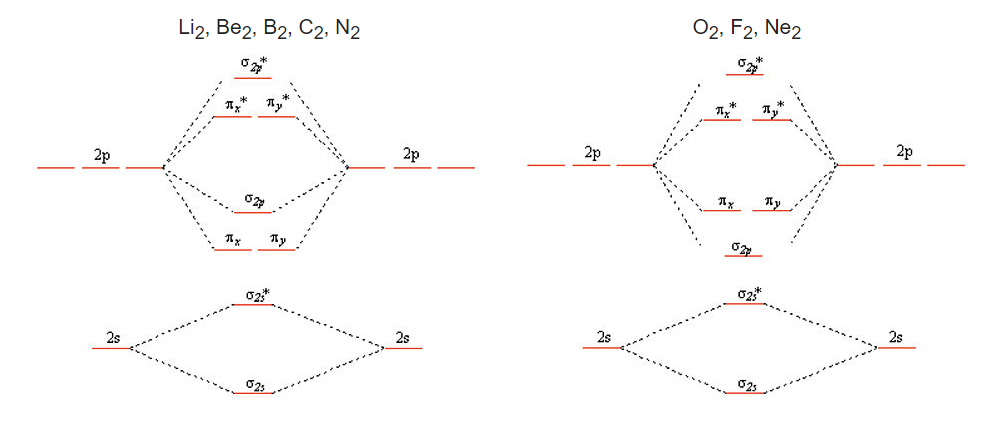
We get the simpler diatomic MO picture on the right when the 2s and 2p atomic orbitals are well separated in energy, as they are for O, F, and Ne. The picture on the left results from mixing of the σ_2s and σ_2p molecular orbitals, which are close in energy for Li₂, Be₂, B₂, C₂, and N₂. Mixing has two effects: 1 - to push the σ_2s* down in energy; and 2 - to push the σ_2p up in energy to the point where the pπ orbitals are below the σ_2p.

Mixing does not occur for O₂ and F₂ because of the energies of the σ_2s and σ_2p molecular orbitals, which are not drawn to scale in the simple picture above. As we move across the second row of the periodic table from Li to F, we are progressively adding protons to the nucleus. The 2s orbital, which has finite amplitude at the nucleus, "feels" the increased nuclear charge more than the 2p orbital. This means that as we progress across the periodic table (and also when we move down the periodic table), the energy difference between the s and p orbitals increases. As the 2s and 2p energies become farther apart in energy, there is less interaction between the orbitals (i.e., less mixing).

A plot of orbital energies is shown below. Because of the very large energy difference between the 1s and 2s/2p orbitals, we plot them on different energy scales, with the 1s to the left and the 2s/2p to the right. For elements at the left side of the 2nd period (Li, Be, B) the 2s and 2p energies are only a few eV apart. The energy difference becomes very large - more than 20 electron volts - for O and F. Since single bond energies are typically about 3-4 eV, this energy difference would be very large on the scale of our MO diagrams. For all the elements in the 2nd row of the periodic table, the 1s (core) orbitals are very low in energy compared to the 2s/2p (valence) orbitals, so we don't need to consider them in drawing our MO diagrams.

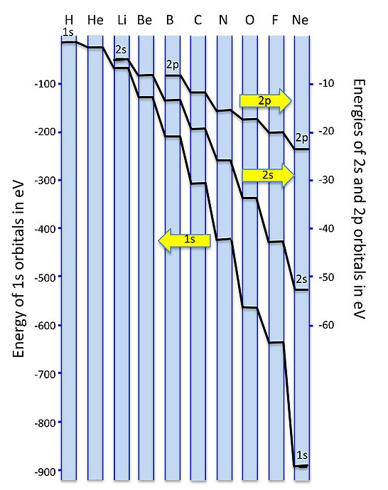Figure \(\PageIndex{1}\): Energies of 1s, 2s, and 2p atomic orbitals for Period 1 and 2 Elements (CC-BY-SA 4.0, Chemistry 310)

Orbital mixing has significant consequences for the magnetic and spectroscopic properties of second period homonuclear diatomic molecules because it affects the order of filling of the \(\sigma_g(2p)\) and \(\pi_u(2p)\) orbitals. Early in period 2 (up to and including nitrogen), the \(\pi_u(2p)\) orbitals are lower in energy than the \(\sigma_g(2p)\) (see Figure \(\PageIndex{1})\). However, later in period 2, the \(\sigma_g(2p)\) orbitals are pulled to a lower energy. This lowering in energy of \(\sigma_g(2p)\) is not unique; all of the \(\sigma\) orbitals in the molecule are pulled to lower energy due to the increasing positive charge of the nucleus. The \(\pi\) orbitals in the molecule are also affected, but to a much lesser extent than \(\sigma\) orbitals. The reason has to do with the high penetration of \(s\) atomic orbitals compared to \(p\) atomic orbitals. The \(\sigma\) molecular orbitals have more \(s\) character and thus their energy is more influenced by increasing nuclear charge. As nuclear charge increases, the energy of the \(\sigma_g(2p)\) orbital is lowered significantly more than the energy of the \(\pi_u(2p)\) orbitals (Figure \(\PageIndex{1})\).

Figure \(\PageIndex{1}\): Molecular orbital energy-level diagrams for the diatomic molecules of the period 2 elements. Unlike earlier diagrams, only the valence molecular orbital energy levels for the molecules are shown here (atomic orbitals not shown for simplicity). For Li₂ through N₂, the \( \sigma _g(2p) \) orbital is higher in energy than the \( \pi_u(2p) \) orbitals. In contrast, from O₂ onward, the \( \sigma _g(2p) \) orbital is lower in energy than the \( \pi_u(2p) \) orbitals because the nuclear charge increases across the row. The experimental bond lengths correlate with the calculated bond order. (CC-BY-NC-SA, Kathryn Haas)

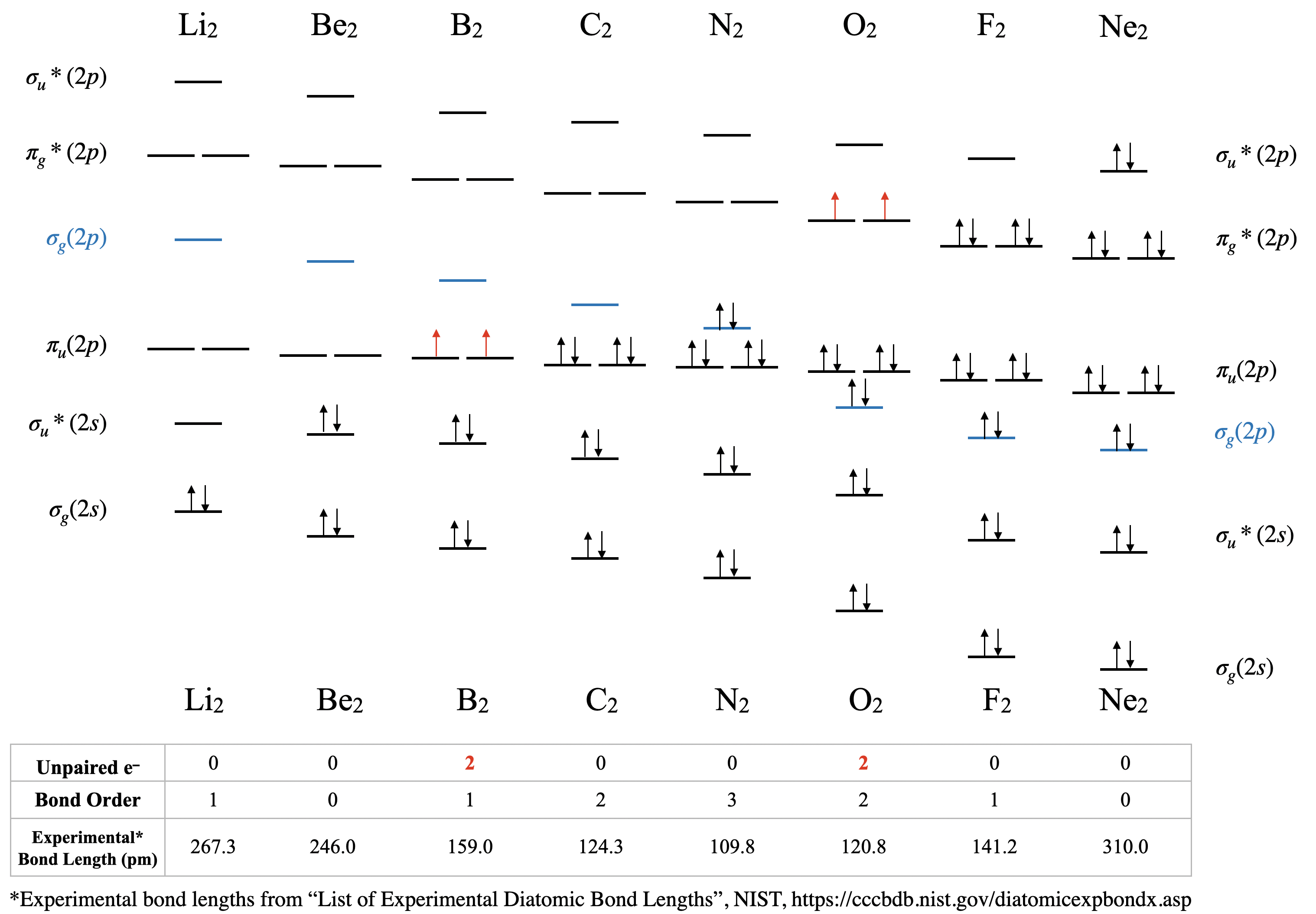
Dilithium, Li₂ \([\sigma_g^2(2s)]\): This molecule has a bond order of one and is observed experimentally in the gas phase to have one Li-Li bond.

Diberylium, Be₂ \([\sigma_g^2\sigma_u^{*2}(2s)]\): This molecule has a bond order of zero due to the equal number of electrons in bonding and antibonding orbitals. Although Be₂ does not exist under ordinary conditions, it can be produced in a laboratory and its bond length measured (Figure \(\PageIndex{2}\)). Although the bond is very weak, its bond length is surprisingly ordinary for a covalent bond of the second period elements.²

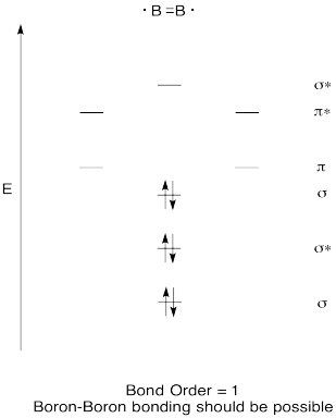
Diboron, B₂ \([\sigma_g^2\sigma_u^{*2}(2s)\pi_u^1\pi_u^1(2p)]\): The case of diboron is one that is much better described by molecular orbital theory than by Lewis structures or valence bond theory. This molecule has a bond order of one. The molecular orbital description of diboron also predicts, accurately, that diboron is paramagnetic. The paramagnetism is a consequence of orbital mixing, resulting in the \(\sigma_g\) orbital's being at a higher energy than the two degenerate \(\pi_u^*\) orbitals.

Dicarbon, C₂ \([\sigma_g^2\sigma_u^{*2}(2s)\pi_u^2\pi_u^2(2p)]\): This molecule has a bond order of two. Molecular orbital theory predicts two bonds with \(\pi\) symmetry, and no \(\sigma\) bonding. C₂ is rare in nature because its allotrope, diamond, is much more stable.

Dinitrogen, N₂ \([\sigma_g^2\sigma_u^{*2}(2s)\pi_u^2\pi_u^2\sigma_g^2(2p)]\): This molecule is predicted to have a triple bond. This prediction is consistent with its short bond length and bond dissociation energy. The energies of the \(\sigma_g(2p)\) and \(\pi_u(2p)\) orbitals are very close, and their relative energy levels have been a subject of some debate (see next section for discussion).

Dioxygen, O₂ \([\sigma_g^2\sigma_u^{*2}(2s)\sigma_g^2\pi_u^2\pi_u^2\pi_g^{*1}\pi_g^{*1}(2p)]\): This is another case where valence bond theory fails to predict actual properties. Molecular orbital theory correctly predicts that dioxygen is paramagnetic, with a bond order of two. Here, the molecular orbital diagram returns to its "normal" order of orbitals where orbital mixing could be somewhat ignored, and where \(\sigma_g(2p)\) is lower in energy than \(\pi_u(2p)\).

Difluorine, F₂ \([\sigma_g^2\sigma_u^{*2}(2s)\sigma_g^2\pi_u^2\pi_u^2\pi_g^{*2}\pi_g^{*2}(2p)]\): This molecule has a bond order of one and like oxygen, the \(\sigma_g(2p)\) is lower in energy than \(\pi_u(2p)\).

Dineon, Ne₂ \([\sigma_g^2\sigma_u^{*2}(2s)\sigma_g^2\pi_u^2\pi_u^2\pi_g^{*2}\pi_g^{*2}\sigma_u^{*2}(2p)]\): Like other noble gases, Ne exists in the atomic form and does not form bonds at ordinary temperatures and pressures. Like Be₂, Ne₂ is an unstable species that has been created in extreme laboratory conditions and its bond length has been measured (Figure \(\PageIndex{2}\)).

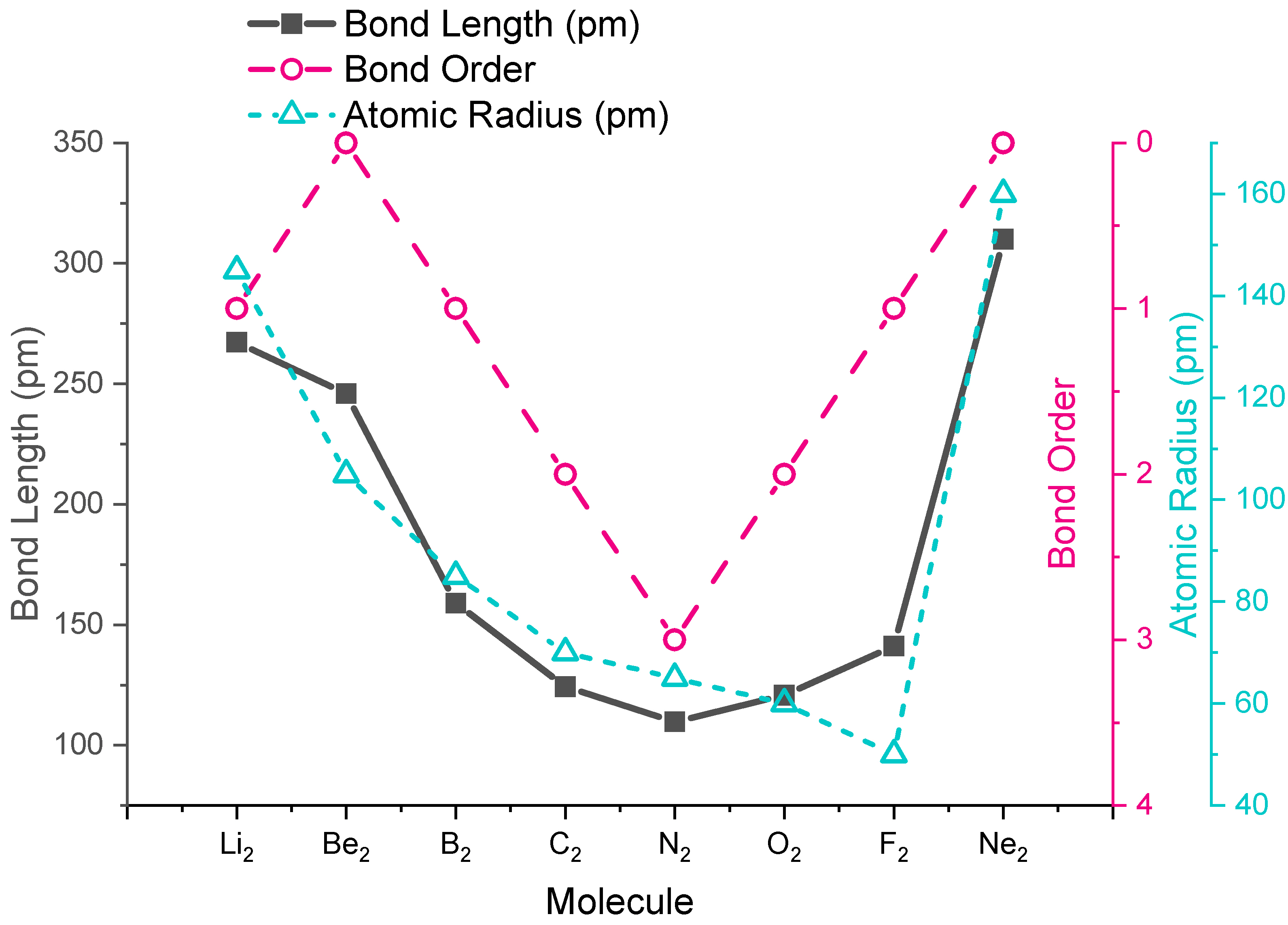
Bond Lengths in Homonuclear Diatomic Molecules

The trends in experimental bond lengths are predicted by molecular orbital theory, specifically by the calculated bond order. The values of bond order and experimental bond lengths for the second period diatomic molecules are given in Figure \(\PageIndex{1}\), and shown in graphical format on the plot in Figure \(\PageIndex{2}\). From the plot, we can see that bond length correlates well with bond order, with a minimum bond length occurring where the bond order is greatest (\(\ce{N2}\)). The shortest bond distance is at \(\ce{N2}\) due to its high bond order of 3. From \(\ce{N2}\) to \(\ce{F2}\) the bond distance increases despite the fact that atomic radius decreases.

Figure \(\PageIndex{2}\): Overlayed plots of bond length (black squares), bond order (pink circles), and atomic radius (teal triangles) versus atomic number for second period homonuclear diatomic molecules. (CC-BY-NC-SA; Kathryn Haas)

Problems

Exercise \(\PageIndex{2}\)

Draw the complete molecular orbital diagrams for \(\ce{H2}\) and for \(\ce{He2}\). Include sketches of the atomic and molecular orbitals.

Answer

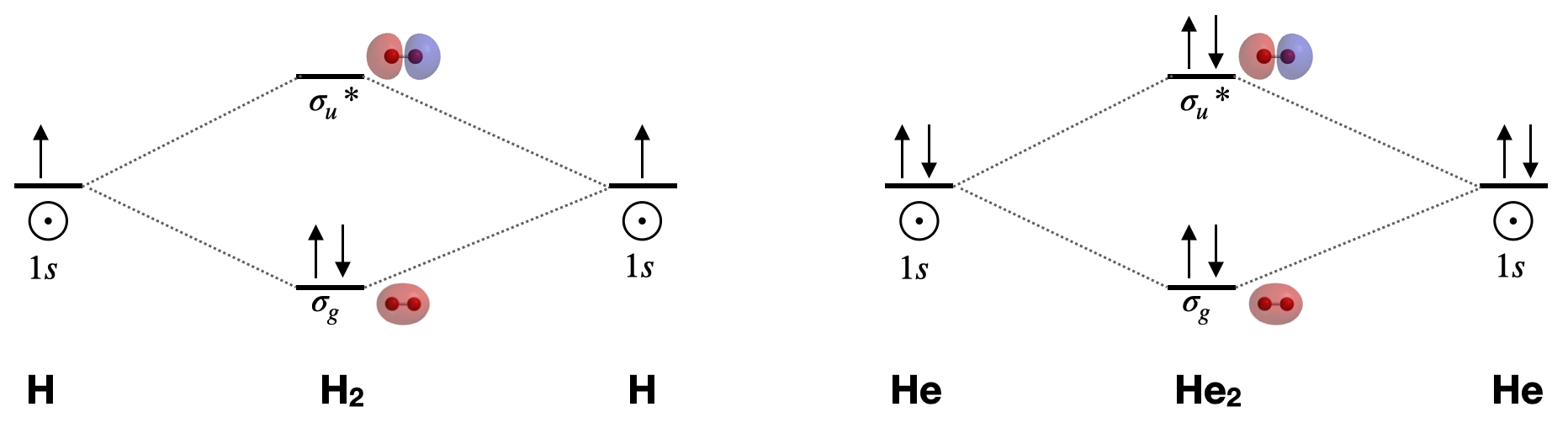
Figure for Exercise \(\PageIndex{1}\): Molecular orbital diagrams for dihydrogen and dihelium. Molecular orbital surfaces calculated using Spartan software. (CC-BY-NC-SA; Kathryn Haas)

A complete molecular orbital diagram includes all atomic orbitals and molecular orbitals, their symmetry labels, and electron filling.

Exercise \(\PageIndex{2}\)

Draw the complete molecular orbital diagram for O₂. Show calculation of its bond order and tell whether it is diamagnetic or paramagnetic.

Answer

O₂ is paramagnetic with a bond order of 2. Its \(\sigma_g(2p)\) molecular orbital is lower in energy that the set of \(\pi_{u}(2p)\) orbitals.

Bond order \(=\frac{1}{2}\left[\left(\begin{array}{c}\text { 8 electrons in} \\ \text { valence bonding orbitals }\end{array}\right)-\left(\begin{array}{c}\text {4 electrons in} \\ \text { valence antibonding orbitals }\end{array}\right)\right]\)

Figure for Exercise \(\PageIndex{2}\). Molecular orbital diagram of O₂. (CC-BY-NC-SA, Kathryn Haas)

Exercise \(\PageIndex{3}\): The Peroxide Ion

Use a qualitative molecular orbital energy-level diagram to predict the electron configuration, the bond order, and the number of unpaired electrons in the peroxide ion (O₂²⁻).

Answer

This diagram looks similar to that of \(\ce{O2}\), except that there are two additional electrons.
\( \left ( \sigma _{g}(2s) \right )^{2}\left ( \sigma_u ^{\star }(2s) \right )^{2}\left ( \sigma _g(2p) \right )^{2}\left ( \pi _{u}(2p) \right )^{4}\left ( \pi _g(2p) \right )^{4} \); bond order of 1; no unpaired electrons.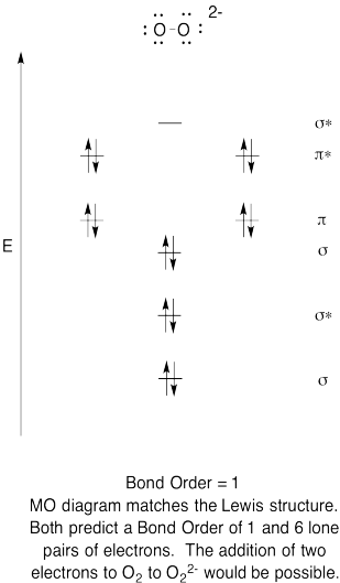

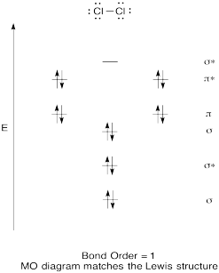
Exercise \(\PageIndex{4}\)

Construct a qualitative molecular orbital diagram for chlorine, Cl₂. Compare the bond order to that seen in the Lewis structure (remember that an electron in an antibonding orbital cancels the stabilization due to bonding of an electron in a bonding orbital).

Answer

Exercise \(\PageIndex{5}\)

Construct a qualitative molecular orbital diagram for diboron, B₂. Do you think boron-boron bonds could form easily, based on this picture?

Answer

Exercise \(\PageIndex{6}\)

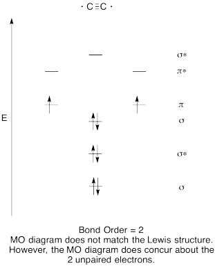
1. Construct a qualitative molecular orbital diagram for dicarbon, C₂.
2. Compare the bond order to that seen in the Lewis structure.
3. How else does this MO picture of oxygen compare to the Lewis structure? What do the two structures tell you about electron pairing?

Answer

Exercise \(\PageIndex{7}\)

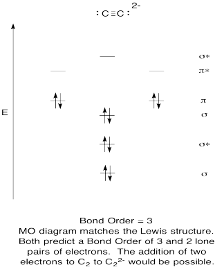
1. Construct a qualitative molecular orbital diagram for acetylide anion, C₂^2-.
2. Compare the bond order to that seen in the Lewis structure.
3. How else does this MO picture of oxygen compare to the Lewis structure? What do the two structures tell you about electron pairing?
4. Based on molecular orbital pictures, how easily do you think dicarbon could be reduced to acetylide (through the addition of two electrons)?

Answer

Exercise \(\PageIndex{8}\)

Make drawings and notes to summarize the effect of populating antibonding orbitals.

Answer

Exercise \(\PageIndex{9}\)

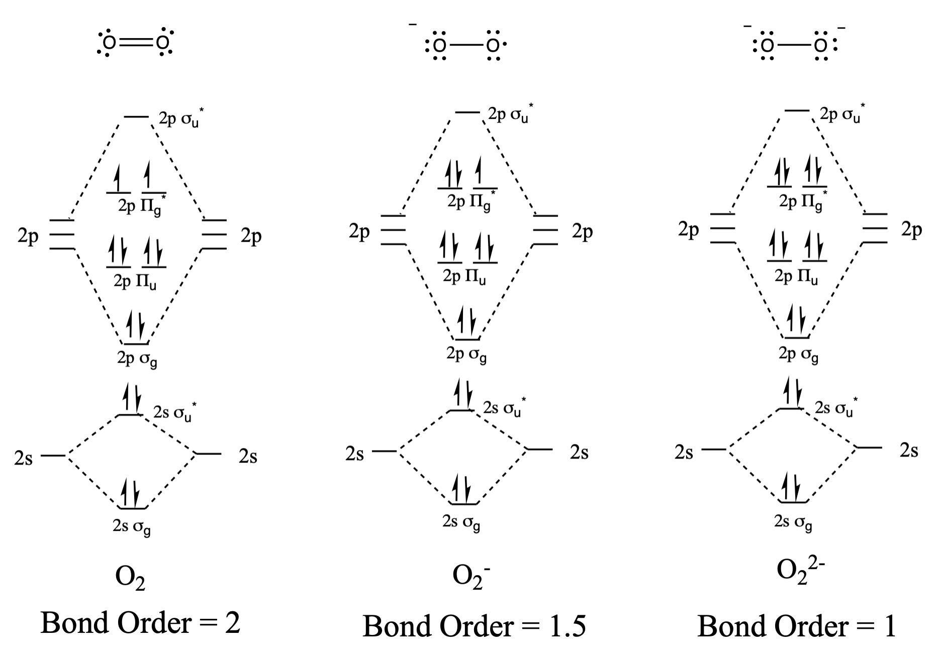
Draw and compare the molecular orbital diagrams to the Lewis structure diagrams for \(\ce{O2}\), \(\ce{O2^-}\), and \(\ce{O2^2-}\).

Answer

The Lewis structures and MO diagrams are shown below. In general, the bond order derived from the MO diagram agrees with the Lewis structure for each species. In the case of the two ions, the number of unpaired electrons from MO theory and the Lewis structure also agrees. In the case of dioxygen, however, there is an inconsistency between the Lewis representation and the MO diagram. While the Lewis structure would lead us to believe that all electrons are paired, the MO diagram indicates paramagnetism, with two unpaired electrons. The MO diagram explains the magnetic behaviour of dioxygen.

References

1. NIST, Calculated Geometries available for H₂⁺ (Hydrogen cation) 2Σg+ D∞h, available at https://cccbdb.nist.gov/diatomicexpbondx.asp
2. Merritt, J. M.; Bondybey, V. E.; Heaven, M. C., Beryllium Dimer-Caught in the Act of Bonding. Science 2009, 324 (5934), 1548-1551.