14.1: Optimizing the Experimental Procedure

In the presence of H₂O₂ and H₂SO₄, a solution of vanadium forms a reddish brown color that is believed to be a compound with the general formula (VO)₂(SO₄)₃. The intensity of the solution’s color depends on the concentration of vanadium, which means we can use its absorbance at a wavelength of 450 nm to develop a quantitative method for vanadium.

The intensity of the solution’s color also depends on the amounts of H₂O₂ and H₂SO₄ that we add to the sample—in particular, a large excess of H₂O₂ decreases the solution’s absorbance as it changes from a reddish brown color to a yellowish color.¹ Developing a standard method for vanadium based on this reaction requires that we optimize the additions of H₂O₂ and H₂SO₄ to maximize the absorbance at 450 nm. Using the terminology of statisticians, we call the solution’s absorbance the system’s response. Hydrogen peroxide and sulfuric acid are factors whose concentrations, or factor levels, determine the system’s response. To optimize the method we need to find the best combination of factor levels. Usually we seek a maximum response, as is the case for the quantitative analysis of vanadium as (VO)₂(SO₄)₃. In other situations, such as minimizing an analysis’s percent error, we are looking for a minimum response.

Note

We will return to this analytical method for vanadium in Example 14.4 and in Problem 14.11.

14.1.1 Response Surfaces

One of the most effective ways to think about an optimization is to visualize how a system’s response changes when we increase or decrease the levels of one or more of its factors. We call a plot of the system’s response as a function of the factor levels a response surface. The simplest response surface has only one factor and is displayed graphically in two dimensions by placing the response on the y-axis and the factor’s levels on the x-axis. The calibration curve in Figure 14.1 is an example of a one-factor response surface. We also can define the response surface mathematically. The response surface in Figure 14.1, for example, is

\[A = 0.008 + 0.0896C_\ce{A}\]

where A is the absorbance and C_A is the analyte’s concentration in ppm.

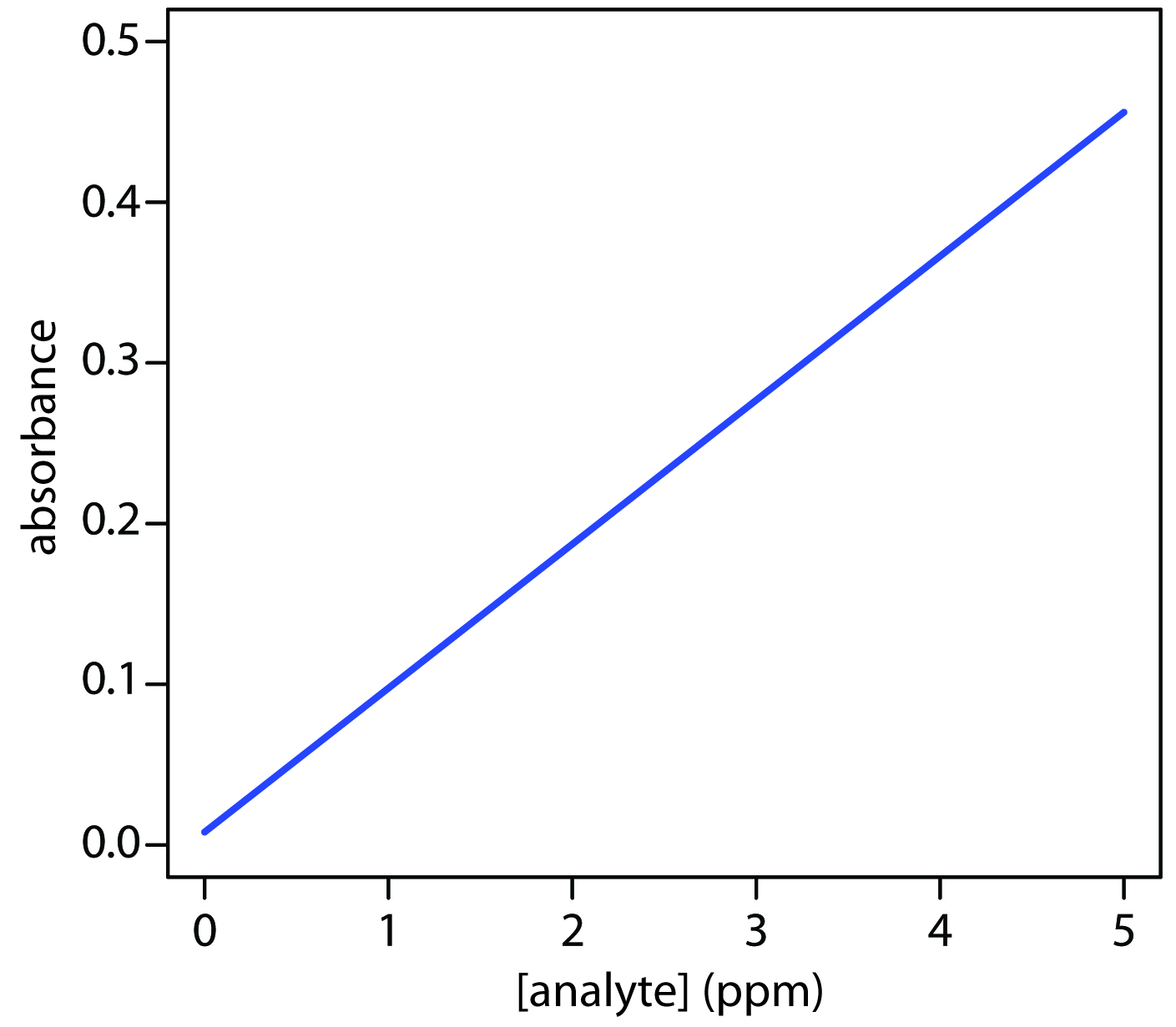
Figure 14.1 A calibration curve is an example of a one-factor response surface. The response (absorbance) is plotted on the y-axis and the factor levels (concentration of analyte) is plotted on the x-axis.

For a two-factor system, such as the quantitative analysis for vanadium described earlier, the response surface is a flat or curved plane in three dimensions. As shown in Figure 14.2a, we place the response on the z-axis and the factor levels on the x-axis and the y-axis. Figure 14.2a shows a pseudo-three dimensional wireframe plot for a system obeying the equation

\[R = 3.0 − 0.30A + 0.020AB\]

where R is the response, and A and B are the factors. We can also represent a two-factor response surface using the two-dimensional level plot in Figure 12.4b, which uses a color gradient to show the response on a two-dimensional grid, or using the two-dimensional contour plot in Figure 14.2c, which uses contour lines to display the response surface.

Note

We also can overlay a level plot and a contour plot. See Figure 14.7b for a typical example.

Figure 14.2 Three examples of a two-factor response surface displayed as (a) a pseudo-three-dimensional wireframe plot, (b) a two-dimensional level plot, and (c) a two-dimensional contour plot. We call the display in (a) a pseudo-three dimensional response surface because we show the presence of three dimensions on the page’s flat, two-dimensional surface.

The response surfaces in Figure 14.2 cover a limited range of factor levels (0 ≤ A ≤ 10, 0 ≤ B ≤ 10), but we can extend each to more positive or more negative values because there are no constraints on the factors. Most response surfaces of interest to an analytical chemist have natural constraints imposed by the factors or have practical limits set by the analyst. The response surface in Figure 14.1, for example, has a natural constraint on its factor because the analyte’s concentration cannot be smaller than zero.

Note

We express this constraint as C_A ≥ 0.

If we have an equation for the response surface, then it is relatively easy to find the optimum response. Unfortunately, we rarely know any useful details about the response surface. Instead, we must determine the response surface’s shape and locate the optimum response by running appropriate experiments. The focus of this section is on useful experimental designs for characterizing response surfaces. These experimental designs are divided into two broad categories: searching methods, in which an algorithm guides a systematic search for the optimum response, and modeling methods, in which we use a theoretical or empirical model of the response surface to predict the optimum response.

14.1.2 Searching Algorithms for Response Surfaces

Figure 14.3 shows a portion of the South Dakota Badlands, a landscape that includes many narrow ridges formed through erosion. Suppose you wish to climb to the highest point of this ridge. Because the shortest path to the summit is not obvious, you might adopt the following simple rule—look around you and take a step in the direction that has the greatest change in elevation. The route you follow is the result of a systematic search using a searching algorithm. Of course there are as many possible routes as there are starting points, three examples of which are shown in Figure 14.3. Note that some routes do not reach the highest point—what we call the global optimum. Instead, many routes reach a local optimum from which further movement is impossible.

Note

Searching algorithms have names—the one described here is the method of steepest ascent.

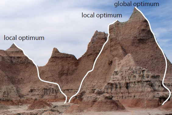
Figure 14.3 Finding the highest point on a ridge using a searching algorithm is one useful model for finding the optimum on a response surface. The path on the far right reaches the highest point, or the global optimum. The other two paths reach local
optima. This ridge is part of the South Dakota Badlands National Park. You can read about the geology of the park as www.nps.gov/badl/.

We can use a systematic searching algorithm to locate the optimum response for an analytical method. We begin by selecting an initial set of factor levels and measure the response. Next, we apply the rules of our searching algorithm to determine a new set of factor levels, continuing this process until we reach an optimum response. Before we consider two common searching algorithms, let’s consider how we evaluate a searching algorithm.

Effectiveness and Efficiency

A searching algorithm is characterized by its effectiveness and its efficiency. To be effective, a searching algorithm must find the response surface’s global optimum, or at least reach a point near the global optimum. A searching algorithm may fail to find the global optimum for several reasons, including a poorly designed algorithm, uncertainty in measuring the response, and the presence of local optima. Let’s consider each of these potential problems.

A poorly designed algorithm may prematurely end the search before it reaches the response surface’s global optimum. As shown in Figure 14.4, an algorithm for climbing a ridge that slopes to the northeast is likely to fail if it allows you to take steps only to the north, south, east, or west. An algorithm must be that responds to a change in the direction of steepest ascent is effective.

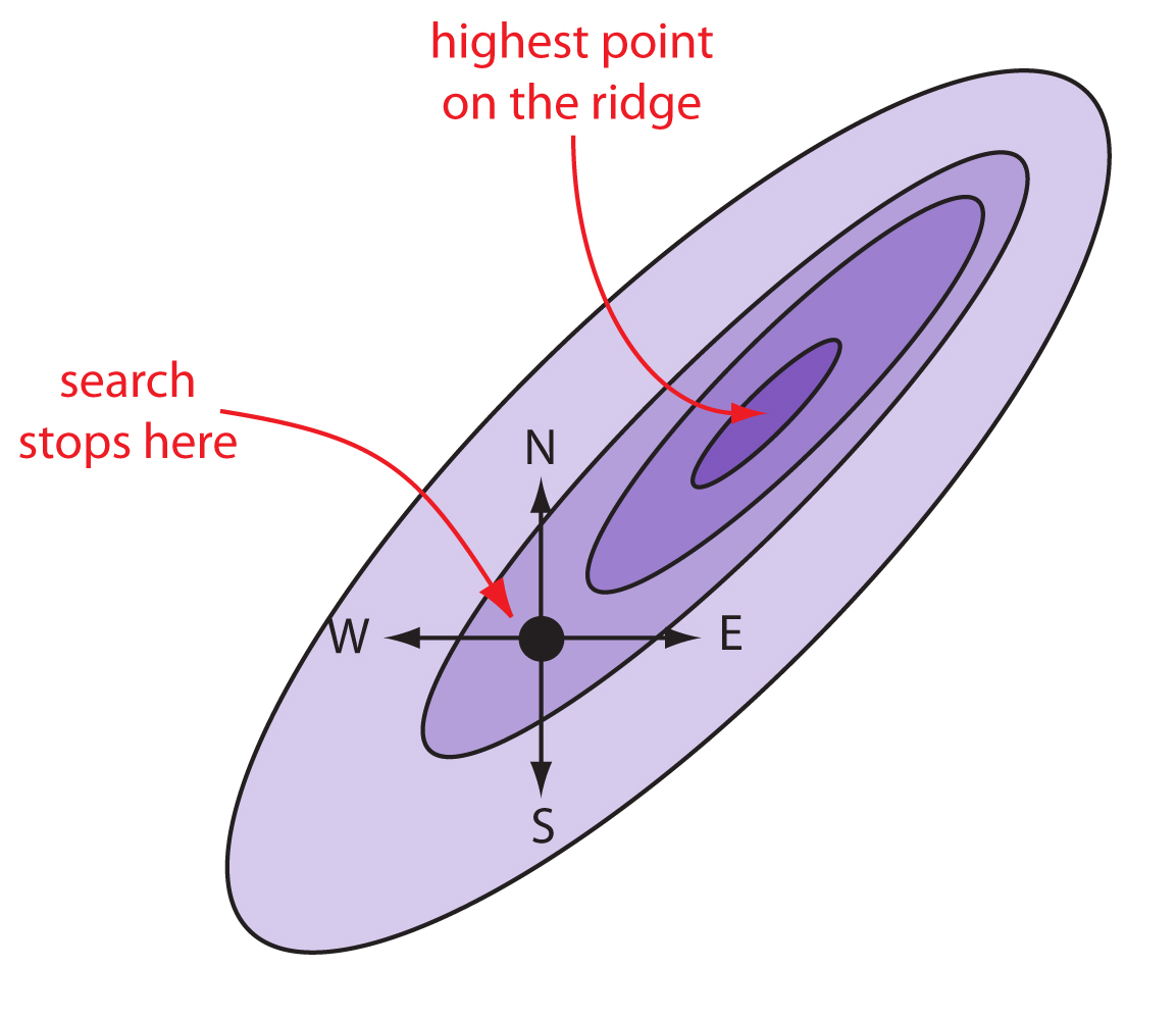
Figure 14.4 Example showing how a poorly designed searching algorithm can fail to find a response surface’s global optimum.

All measurements contain uncertainty, or noise, that affects our ability to characterize the underlying signal. When the noise is greater than the local change in the signal, then a searching algorithm is likely to end before it reaches the global optimum. Figure 14.5 provides a different view of Figure 14.3, showing us that the relatively flat terrain leading up to the ridge is heavily weathered and uneven. Because the variation in local height exceeds the slope, our searching algorithm stops the first time we step up onto a less weathered surface.

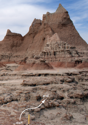
Figure 14.5 Another view of the ridge in Figure 14.3 showing the weathered terrain leading up to the ridge. The yellow rod at the bottom of the figure, which marks a trail, is about 18 in high.

Finally, a response surface may contain several local optima, only one of which is the global optimum. If we begin the search near a local optimum, our searching algorithm may not be capable of reaching the global optimum. The ridge in Figure 14.3, for example, has many peaks. Only those searches beginning at the far right reach the highest point on the ridge. Ideally, a searching algorithm should reach the global optimum regardless of where it starts.

A searching algorithm always reaches an optimum. Our problem, of course, is that we do not know if it is the global optimum. One method for evaluating a searching algorithm’s effectiveness is to use several sets of initial factor levels, finding the optimum response for each, and comparing the results. If we arrive at the same optimum response after starting from very different locations on the response surface, then we are more confident that is it the global optimum.

Efficiency is the second desirable characteristic for a searching algorithm. An efficient algorithm moves from the initial set of factor levels to the optimum response in as few steps as possible. We can increase the rate at which we approach the optimum by taking larger steps. If the step size is too large, however, the difference between the experimental optimum and the true optimum may be unacceptably large. One solution is to adjust the step size during the search, using larger steps at the beginning and smaller steps as we approach the global optimum.

One-Factor-at-a-Time Optimization

A simple algorithm for optimizing the quantitative method for vanadium described earlier is to select initial concentrations for H₂O₂ and H₂SO₄ and measure the absorbance. Next, we optimize one reagent by increasing or decreasing its concentration—holding constant the second reagent’s concentration—until the absorbance decreases. We then vary the concentration of the second reagent—maintaining the first reagent’s optimum concentration—until we observe a decrease in absorbance. We can stop this process, which we call a one-factor-at-a-time optimization, after one cycle or repeat it until the absorbance reaches a maximum value or it exceeds an acceptable threshold value.

A one-factor-at-a-time optimization is consistent with a notion that to determine the influence of one factor we must hold constant all other factors. This is an effective, although not necessarily an efficient experimental design when the factors are independent.² Two factors are independent when changing the level of one factor does not influence the effect of changing the other factor’s level. Table 14.1 provides an example of two independent factors. If we hold factor B at level B₁, changing factor A from level A₁ to level A₂ increases the response from 40 to 80, or a change in response, ∆R, of

\[R = 80 - 40 = 40\]

If we hold factor B at level B₂, we find that we have the same change in response when the level of factor A changes from A₁ to A₂.

\[R = 100 - 60 = 40\]

We can see this independence graphically by plotting the response versus factor A’s level, as shown in Figure 14.6. The parallel lines show that the level of factor B does not influence factor A’s effect on the response.

Table 14.1 Example of Two Independent Factors

factor A	factor B	response
A1	B1	40
A2	B1	80
A1	B2	60
A2	B2	100

Figure 14.6 Factor effect plot for two independent factors. Note that the two lines are parallel, indicating that the level for factor B does not influence how factor A’s level affects the response.

Practice Exercise 14.1

Using the data in Table 14.1, show that factor B’s affect on the response is independent of factor A.

Click here to review your answer to this exercise.

Mathematically, two factors are independent if they do not appear in the same term in the equation describing the response surface. Equation 14.1, for example, describes a response surface with independent factors because no term in the equation includes both factor A and factor B.

\[R = 2.0 + 0.12A + 0.48B - 0.03A^2 - 0.03B^2\tag{14.1}\]

Figure 14.7 shows the resulting pseudo-three-dimensional surface and a contour map for equation 14.1.

The easiest way to follow the progress of a searching algorithm is to map its path on a contour plot of the response surface. Positions on the response surface are identified as (a, b) where a and b are the levels for factors A and B. The contour plot in Figure 14.7b, for example, shows four one-factor-at-a-time optimizations of the response surface for equation 14.1. The effectiveness and efficiency of this algorithm when optimizing independent factors is clear—each trial reaches the optimum response at (2, 8) in a single cycle.

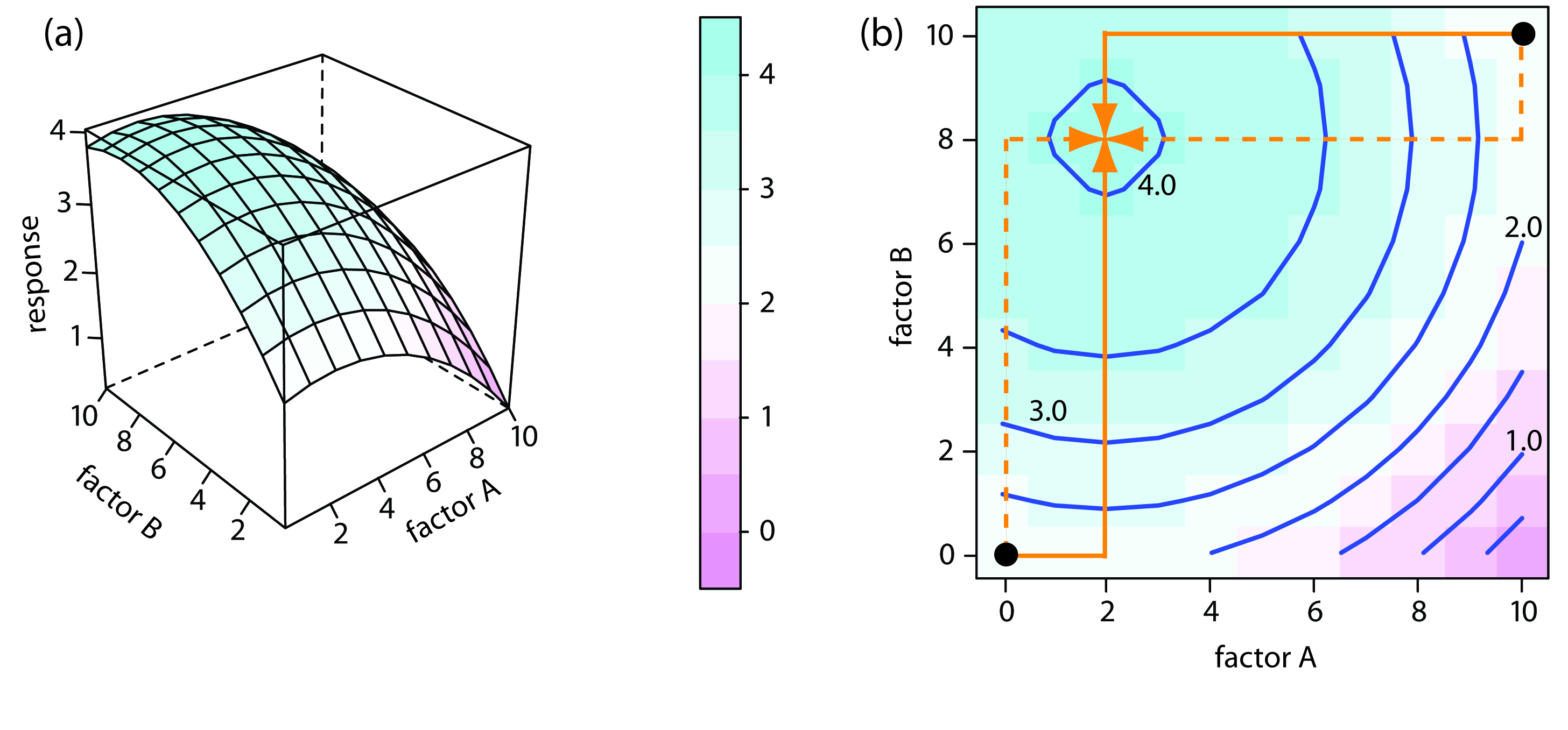
Figure 14.7 The response surface for two independent factors based on equation 14.1, displayed as (a) a wireframe, and (b) an overlaid contour plot and level plot. The orange lines in (b) show the progress of one-factor-at-a-time optimizations beginning from two starting points (•) and optimizing factor A first (solid line) or factor B first (dashed line). All four trials reach the optimum response of (2,8) in a single cycle.

Unfortunately, factors usually do not behave independently. Consider, for example, the data in Table 14.2. Changing the level of factor B from level B₁ to level B₂ has a significant effect on the response when factor A is at level A₁

\[R = 60 - 20 = 40\]

but no effect when factor A is at level A₂.

\[R = 80 - 80 = 0\]

Table 14.2 Example of Two Dependent Factors

factor A	factor B	response
A1	B1	20
A2	B1	80
A1	B2	60
A2	B2	80

Figure 14.8 shows this dependent relationship between the two factors. Factors that are dependent are said to interact and the response surface’s equation includes an interaction term containing both factors A and B. The final term in equation 14.2, for example, accounts for the interaction between the factors A and B.

\[R = 5.5 + 1.5A + 0.6B - 0.15A^2 - 0.0245B^2 - 0.0857AB\tag{14.2}\]

Figure 14.8 Factor effect plot for two dependent factors. Note that the two lines are not parallel, indicating that the level for factor A influences how factor B’s level affects the response.

Figure 14.9 shows the resulting pseudo-three-dimensional surface and a contour map for equation 14.2.

The progress of a one-factor-at-a-time optimization for equation 14.2 is shown in Figure 14.9b. Although the optimization for dependent factors is effective, it is less efficient than that for independent factors. In this case it takes four cycles to reach the optimum response of (3, 7) if we begin at (0, 0).

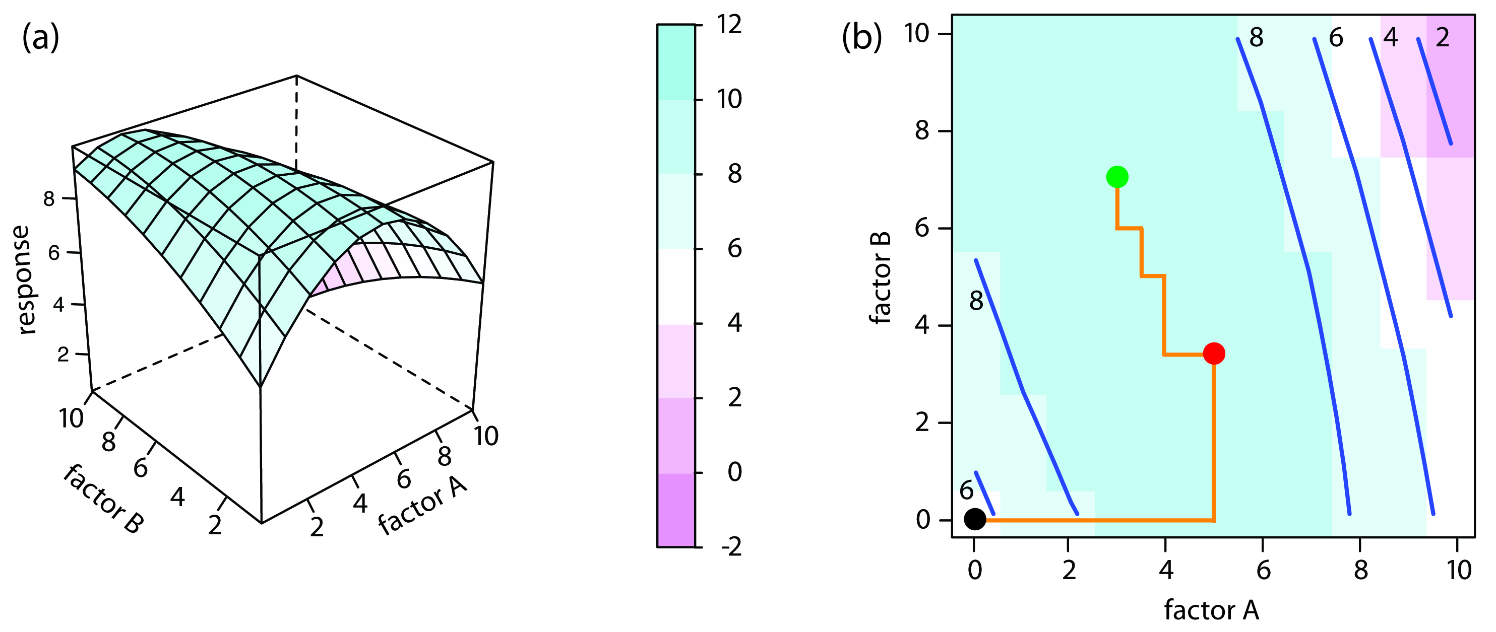
Figure 14.9 The response surface for two dependent factors based on equation 14.2, displayed as (a) a wireframe, and (b) an overlaid contour plot and level plot. The orange lines in (b) show the progress of one-factor-at-a-time optimization beginning from the starting point (•) and optimizing factor A first. The red dot (•) marks the end of the first cycle. It takes four cycles to reach the optimum response of (3, 7) as shown by the green dot (•).

Practice Exercise 14.2

Using the data in Table 14.2, show that factor A’s affect on the response is independent of factor B.

Click here to review your answer to this exercise.

Simplex Optimization

One strategy for improving the efficiency of a searching algorithm is to change more than one factor at a time. A convenient way to accomplish this when there are two factors is to begin with three sets of initial factor levels, which form the vertices of a triangle. After measuring the response for each set of factor levels, we identify the combination giving the worst response and replace it with a new set of factor levels using a set of rules (Figure 14.10). This process continues until we reach the global optimum or until no further optimization is possible. The set of factor levels is called a simplex. In general, for k factors a simplex is a k + 1 dimensional geometric figure.³

Note

Thus, for two factors the simplex is a triangle. For three factors the simplex is a tetrahedron.

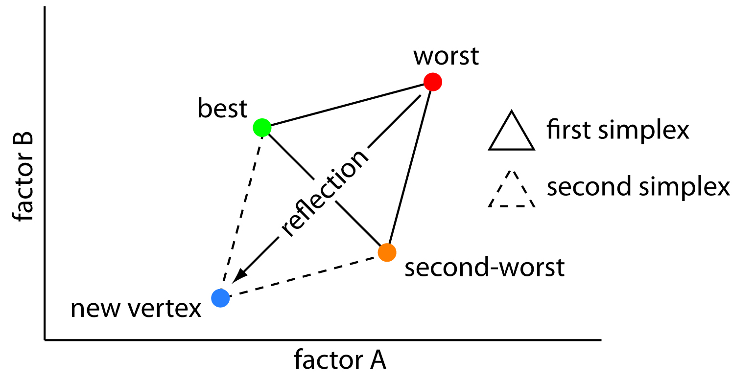
Figure 14.10 Example of a two-factor simplex. The original simplex is formed by the green, orange, and red vertices. Replacing the worst vertex with a new vertex moves the simplex into a new position on the response surface.

To place the initial two-factor simplex on the response surface, we choose a starting point (a, b) for the first vertex and place the remaining two vertices at (a + s_a, b) and (a + 0.5s_a, b + 0.87s_b) where s_a and s_b are step sizes for factors A and B.⁴ The following set of rules moves the simplex across the response surface in search of the optimum response:

Rule 1. Rank the vertices from best (v_b) to worst (v_w).

Rule 2. Reject the worst vertex (v_w) and replace it with a new vertex (v_n) by reflecting the worst vertex through the midpoint of the remaining vertices. The new vertex’s factor levels are twice the average factor levels for the retained vertices minus the factor levels for the worst vertex. For a two-factor optimization, the equations are shown here where v_s is the third vertex.

\[a_{v_n}=2\left(\dfrac{a_{v_\ce{b}}+a_{v_\ce{s}}}{2}\right)-a_{v_\ce{w}}\tag{14.3}\]

\[b_{v_n}=2\left(\dfrac{b_{v_\ce{b}}+b_{v_\ce{s}}}{2}\right)-b_{v_\ce{w}}\tag{14.4}\]

Note

The variables a and b in equation 14.3 and equation 14.4 are the factor levels for factors A and B, respectively. Problem 14.3 in the end-of-chapter problems asks you to derive these equations.

Rule 3. If the new vertex has the worst response, then return to the previous vertex and reject the vertex with the second worst response, (v_s) calculating the new vertex’s factor levels using rule 2. This rule ensures that the simplex does not return to the previous simplex.

Rule 4. Boundary conditions are a useful way to limit the range of possible factor levels. For example, it may be necessary to limit a factor’s concentration for solubility reasons, or to limit the temperature because a reagent is thermally unstable. If the new vertex exceeds a boundary condition, then assign it the worst response and follow rule 3.

Because the size of the simplex remains constant during the search, this algorithm is called a fixed-sized simplex optimization. Example 14.1 illustrates the application of these rules.

Example 14.1

Find the optimum response for the response surface in Figure 14.9 using the fixed-sized simplex searching algorithm. Use (0, 0) for the initial factor levels and set each factor’s step size to 1.00.

Solution

Letting a = 0, b = 0, s_a = 1, and s_b = 1 gives the vertices for the initial simplex as

Vertex 1: (a, b) = (0, 0)

Vertex 2: (a + s_a, b) = (1.00, 0)

Vertex 3: (a + 0.50s_a, b + 0.87s_b) = (0.50, 0.87)

The responses, from equation 14.2, for the three vertices are shown in the following table

vertex	a	b	response
v1	0	0	5.50
v2	1.00	0	6.85
v3	0.50	0.87	6.68

with v₁ giving the worst response and v₃ the best response. Following Rule 1, we reject v₁ and replace it with a new vertex using equation 14.3 and equation 14.4; thus

\[a_{v_4}=2 \times \dfrac{1.00+0.50}{2}-0=1.50 \hspace{5mm}b_{v_4}=2 \times \dfrac{0+0.87}{2}-0=0.87\]

The following table gives the vertices of the second simplex.

vertex	a	b	response
v2	1.50	0	6.85
v3	0.50	0.87	6.68
v4	1.50	0.87	7.80

with v₃ giving the worst response and v₄ the best response. Following Rule 1, we reject v₃ and replace it with a new vertex using equation 14.3 and equation 14.4; thus

\[a_{v_5}=2 \times \dfrac{1.00+1.50}{2}-0.50=2.00 \hspace{5mm}b_{v_5}=2 \times \dfrac{0+0.87}{2}-0.87=0\]

The following table gives the vertices of the third simplex.

vertex	a	b	response
v2	1.50	0	6.85
v4	1.50	0.87	7.80
v5	2.00	0	7.90

The calculation of the remaining vertices is left as an exercise. Figure 14.11 shows the progress of the complete optimization. After 29 steps the simplex begins to repeat itself, circling around the optimum response of (3, 7).

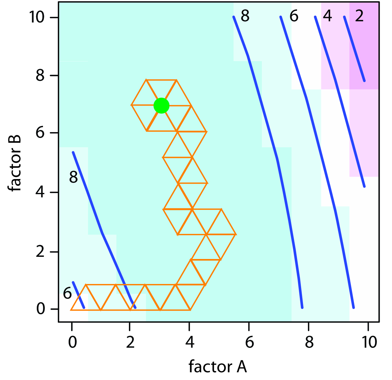
Figure 14.11 Progress of the fixed-size simplex optimization in Example 14.1. The green dot marks the optimum response of (3, 7). Optimization ends when the simplexes begin to circle around a single vertex.

Practice Exercise 14.3

The following exercise will help you evaluate the efficiency and effectiveness of three common searching algorithms: one-factor-at-a-time, fixed-size simplex, and variable-sized simplex (see the following side comment for a brief description and a link to additional information). Click on this link, which opens a java applet. Scroll down to read the applet’s instructions and then experiment with the controls. When you are comfortable with the applet’s interface, answer the following questions: (a) How sensitive is each algorithm to its initial starting point and to the size of the initial simplex or step? In your answer, consider both effectiveness and efficiency. (b) Are the optimizations for some response surfaces particularly sensitive to the initial position? If so, what are the characteristics of these response surfaces?

Click here to review your answer to this exercise.

Note

The size of the initial simplex ultimately limits the effectiveness and the efficiency of a fixed-size simplex searching algorithm. We can increase its efficiency by allowing the size of the simplex to expand or contract in response to the rate at which we are approaching the optimum. For example, if we find that a new vertex is better than any of the vertices in the preceding simplex, then we expand the simplex further in this direction on the assumption that we are moving directly toward the optimum. Other conditions cause us to contract the simplex—making it smaller—to encourage the optimization to move in a different direction. We call this a variable-sized simplex optimization.

Consult this chapter’s additional resources for further details of the variable-sized simplex optimization.

14.1.3 Mathematical Models of Response Surfaces

A response surface is described mathematically by an equation relating the response to its factors. Equation 14.1 and equation 14.2 provide two examples. If we measure the response for several combinations of factor levels, then we can model the response surface by using a linear regression analysis to fit an appropriate equation to the data. There are two broad categories of models that we can use in a regression analysis: theoretical models and empirical models.

Theoretical Models of the Response Surface

A theoretical model is derived from the known chemical and physical relationships between the response and its factors. In spectrophotometry, for example, Beer’s law is a theoretical model that relates a substance’s absorbance, A, to its concentration, C_A

\[A = εbC_\ce{A}\]

where ε is the molar absorptivity and b is the pathlength of the electromagnetic radiation passing through the sample. A Beer’s law calibration curve, therefore, is a theoretical model of a response surface.

Note

For a review of Beer’s law, see Section 10.2.3 in Chapter 10. Figure 14.1 is an example of a Beer’s law calibration curve.

Empirical Models of the Response Surface

In many cases the underlying theoretical relationship between the response and its factors is unknown. We can still develop a model of the response surface if we make some reasonable assumptions about the underlying relationship between the factors and the response. For example, if we believe that the factors A and B are independent and that each has only a first-order effect on the response, then the following equation is a suitable model.

\[R = β_0 + β_aA + β_bB\]

where R is the response, A and B are the factor levels, and β₀, β_a, and β_b are adjustable parameters whose values are determined by a linear regression analysis. Other examples of equations include those for dependent factors

\[R = β_0 + β_aA+ β_bB + β_{ab}AB\]

and those with higher-order terms.

\[R = β_0 + β_aA + β_bB + β_{aa}A^2 + β_{bb}B^2\]

Each of these equations provides an empirical model of the response surface because it has no basis in a theoretical understanding of the relationship between the response and its factors. Although an empirical model may provide an excellent description of the response surface over a limited range of factor levels, it has no basis in theory and cannot be extended to unexplored parts of the response surface.

Note

The calculations for a linear regression when the model is first-order in one factor (a straight line) is described in Chapter 5.4. A complete mathematical treatment of linear regression for models that are second-order in one factor or which contain more than one factor is beyond the scope of this text. The computations for a few special cases, however, are straightforward and are considered in this section. A more comprehensive treatment of linear regression can be found in several of this chapter’s additional resources.

Factorial Designs

To build an empirical model we measure the response for at least two levels for each factor. For convenience we label these levels as high, H_f, and low, L_f, where f is the factor; thus H_A is the high level for factor A and L_B is the low level for factor B. If our empirical model contains more than one factor, then each factor’s high level is paired with both the high level and the low level for all other factors. In the same way, the low level for each factor is paired with the high level and the low level for all other factors. As shown in Figure 14.12, this requires 2^k experiments where k is the number of factors. This experimental design is known as a 2^k factorial design.

Note

Another system of notation is to use a plus sign (+) to indicate a factor’s high level and a minus sign (–) to indicate its low level. We will use H or L when writing an equation and a plus sign or a minus sign in tables.

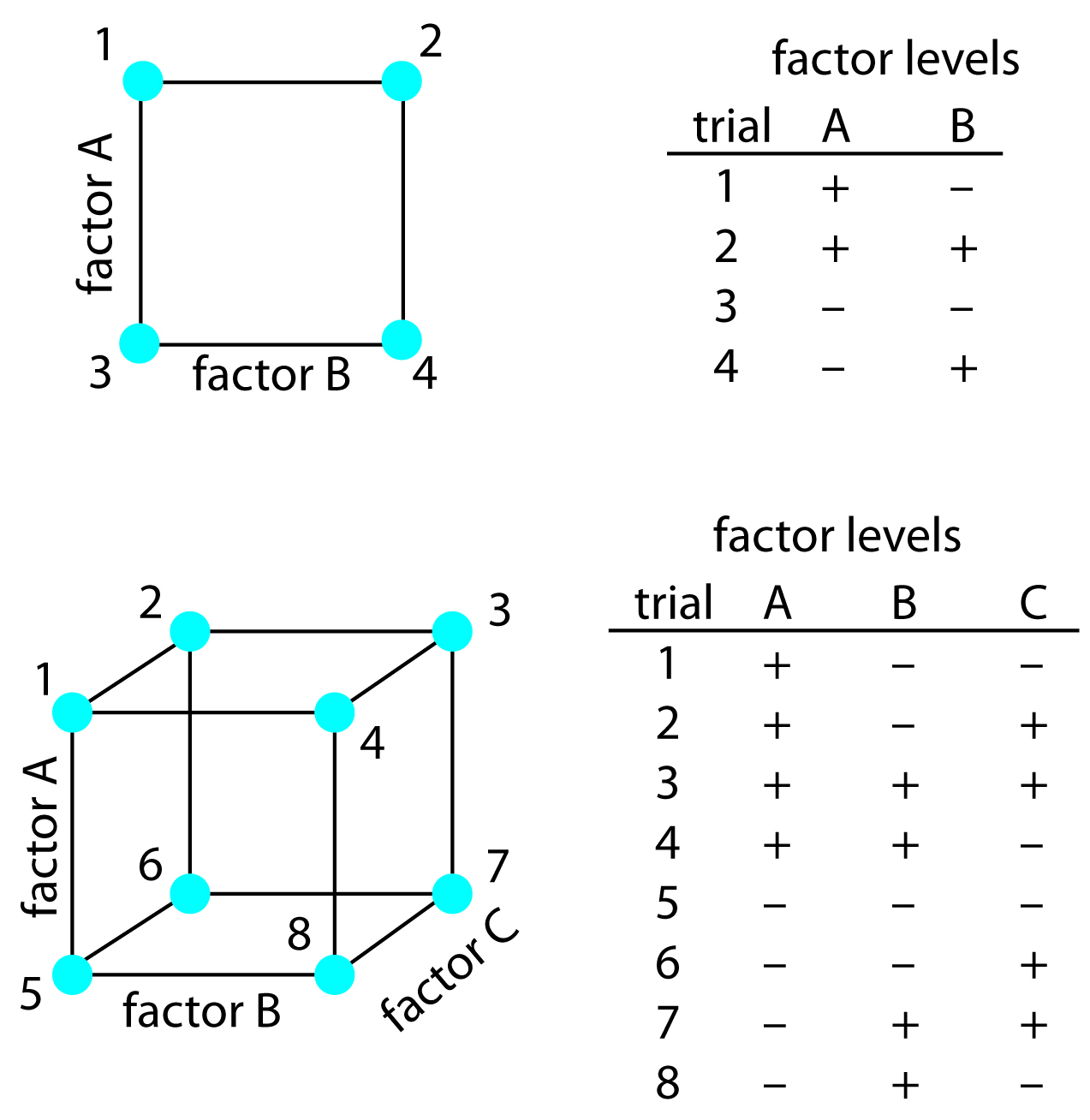
Figure 14.12 2^k factorial designs for (top) k = 2, and (bottom) k = 3. A 2² factorial design requires four experiments and a 2³ factorial design requires eight experiments.

Coded Factor Levels

The calculations for a 2^k factorial design are straightforward and easy to complete with a calculator or spreadsheet. To simplify the calculations, we code the factor levels using +1 for a high level and –1 for a low level. Coding has two additional advantages: scaling the factors to the same magnitude makes it easier to evaluate each factor’s relative importance, and it places the model’s intercept, β₀, at the center of the experimental design. As shown in Example 14.2, it is easy to convert between coded and uncoded factor levels.

Example 14.2

To explore the effect of temperature on a reaction, we assign 30^oC to a coded factor level of –1, and assign a coded level +1 to a temperature of 50^oC. What temperature corresponds to a coded level of –0.5 and what is the coded level for a temperature of 60^oC?

Solution

The difference between –1 and +1 is 2, and the difference between 30^oC and 50^oC is 20^oC; thus, each unit in coded form is equivalent to 10^oC in uncoded form. With this information, it is easy to create a simple scale between the coded and the uncoded values, as shown in Figure 14.13. A temperature of 35^oC corresponding to a coded level of –0.5 and a coded level of +2 corresponds to a temperature of 60^oC.

Figure 14.13 The relationship between the coded factor levels and the uncoded factor levels for Example 14.2. The numbers in red are the values defined in the 2² factorial design.

Determining the Empirical Model

Let’s begin by considering a simple example involving two factors, A and B, and the following empirical model.

\[R = β_0 + β_aA + β_bB + β_{ab}AB\tag{14.5}\]

A 2^k factorial design with two factors requires four runs. Table 14.3 provides the uncoded levels (A and B), the coded levels (A* and B*), and the responses (R) for these experiments. The terms β₀, β_a, β_b, and β_ab in equation 14.5 account for, respectively, the mean effect (which is the average response), first-order effects due to factors A and B, and the interaction between the two factors.

Table 14.3 Example of Uncoded and Coded Factor Levels and Responses for a 2² Factorial Design

run	A	B	A*	B*	R
1	15	30	+1	+1	22.5
2	15	10	+1	–1	11.5
3	5	30	–1	+1	17.5
4	5	10	–1	–1	8.5

Equation 14.5 has four unknowns—the four beta terms—and Table 14.3 describes four experiments. We have just enough information to calculate values for β₀, β_a, β_b, and β_ab. When working with the coded factor levels, the values of these parameters are easy to calculate using the following equations, where n is the number of runs.

\[\beta _0\approx b_0=\frac{1}{n}\sum_{i}R_i\tag{14.6}\]

\[\beta _\ce{a}\approx b_\ce{a}=\frac{1}{n}\sum_{i}A_i^\ast R_i\tag{14.7}\]

\[\beta _\ce{b}\approx b_\ce{b}=\frac{1}{n}\sum_{i}B_i^\ast R_i\tag{14.8}\]

\[\beta _\ce{ab}\approx b_\ce{ab}=\frac{1}{n}\sum_{i}A_i^\ast B_i^\ast R_i\tag{14.9}\]

Note

Recall that we introduced coded factor levels with the promise that they simplify calculations.

In Section 5.4.1 of Chapter 5 we introduced the convention of using β to indicate the true value of a regression’s model’s parameter’s and b to indicate its calculated value. We estimate β from b.

Solving for the estimated parameters using the data in Table 14.3

\[b_0=\dfrac{22.5+11.5+17.5+8.5}{4}=15.0\]

\[b_\ce{a}=\dfrac{22.5+11.5-17.5-8.5}{4}=2.0\]

\[b_\ce{b}=\dfrac{22.5-11.5+17.5-8.5}{4}=5.0\]

\[b_\ce{ab}=\dfrac{22.5-11.5-17.5+8.5}{4}=0.5\]

leaves us with the following coded empirical model for the response surface.

\[R = 15.0 + 2.0A^* + 5.0B^* + 0.5A^*B^*\tag{14.10}\]

Note

Although we can convert this coded model into its uncoded form, there is no need to do so. If we need to know the response for a new set of factor levels, we just convert them into coded form and calculate the response. For example, if A is 10 and B is 15, then A* is 0 and B* is –0.5. Substituting these values into equation 14.10 gives a response of 12.5.

We can extend this approach to any number of factors. For a system with three factors—A, B, and C—we can use a 2³ factorial design to determine the parameters in the following empirical model

\[R = β_0 + β_\ce{a}A+ β_\ce{b}B + β_\ce{c}C + β_\ce{ab}AB+ β_\ce{ac}AC + β_\ce{bc}BC + β_\ce{abc}ABC\tag{14.11}\]

where A, B, and C are the factor levels. The terms β₀, β_a, β_b, and β_ab are estimated using equation 14.6, equation 14.7, equation 14.8, and equation 14.9, respectively. To find estimates for the remaining parameters we use the following equations.

\[\beta_\ce{c}=b_\ce{c}=\frac{1}{n}\sum C_i^\ast R_i\tag{14.12}\]

\[\beta_\ce{ac}=b_\ce{ac}=\frac{1}{n}\sum A_i^\ast C_i^\ast R_i\tag{14.13}\]

\[\beta_\ce{bc}=b_\ce{bc}=\frac{1}{n}\sum B_i^\ast C_i^\ast R_i\tag{14.14}\]

\[\beta_\ce{abc}=b_\ce{abc}=\frac{1}{n}\sum A_i^\ast B_i^\ast C_i^\ast R_i\tag{14.15}\]

Example 14.3

Table 14.4 lists the uncoded factor levels, the coded factor levels, and the responses for a 2³ factorial design. Determine the coded empirical model for the response surface based on equation 14.11. What is the expected response when A is 10, B is 15, and C is 50?

Solution

Equation 14.5 has eight unknowns—the eight beta terms—and Table 14.4 describes eight experiments. We have just enough information to calculate values for β₀, β_a, β_b, β_c, β_ab, β_ac, β_bc, and β_abc; these values are

\[b_0 = \dfrac{1}{8}(137.25 + 54.75 + 73.75 + 30.25 + 61.75 + 30.25 + 41.25 + 18.75) = 56.0\]

(See equation 14.6.)

\[b_\ce{a} = \dfrac{1}{8}(137.25 + 54.75 + 73.75 + 30.25 - 61.75 - 30.25 - 41.25 - 18.75) = 18.0\]

(See equation 14.7.)

\[b_\ce{b} = \dfrac{1}{8}(137.25 + 54.75 - 73.75 - 30.25 + 61.75 + 30.25 - 41.25 - 18.75) = 15.0\]

(See equation 14.8.)

\[b_\ce{c} = \dfrac{1}{8}(137.25 - 54.75 + 73.75 - 30.25 + 61.75 - 30.25 + 41.25 - 18.75) = 22.5\]

(See equation 14.9.)

\[b_\ce{ab} = \dfrac{1}{8}(137.25 + 54.75 - 73.75 - 30.25 - 61.75 - 30.25 + 41.25 + 18.75) = 7.0\]

(See equation 14.12.)

\[b_\ce{ac} = \dfrac{1}{8}(137.25 - 54.75 + 73.75 - 30.25 - 61.75 + 30.25 - 41.25 + 18.75) = 9.0\]

(See equation 14.13.)

\[b_\ce{bc} = \dfrac{1}{8}(137.25 - 54.75 - 73.75 + 30.25 + 61.75 - 30.25 - 41.25 + 18.75) = 6.0\]

(See equation 14.14.)

\[b_\ce{abc} = \dfrac{1}{8}(137.25 - 54.75 - 73.75 + 30.25 - 61.75 + 30.25 + 41.25 - 18.75) = 3.75\]

(See equation 14.15.)

The coded empirical model, therefore, is

\[R = 56.0 + 18.0A^∗ + 15.0B^∗ + 22.5C^∗ + 7.0A^∗B^∗ + 9.0A^∗C^∗ + 6.0B^∗C^∗ + 3.75A^∗B^∗C^∗\]

To find the response when A is 10, B is 15, and C is 50, we first convert these values into their coded form. Figure 14.14 helps us make the appropriate conversions; thus, A* is 0, B* is –0.5, and C* is +1.33. Substituting back into the empirical model gives a response of

\[R = 56.0 + 18.0(0) + 15.0(−0.5) + 22.5(1.33) \\
\hspace{70px}+ 7.0(0)(−0.5) + 9.0(0)(1.33) + 6.0(−0.5)(1.33) \\
\hspace{250px}+ 3.75(0)(−0.5)(1.33) = 74.435\]

Table 14.4 Example of Uncoded and Coded Factor Levels and Responses for the 2³ Factorial Design in Example 14.3

run	A	B	C	A*	B*	C*	R
1	15	30	45	+1	+1	+1	137.25
2	15	30	15	+1	+1	–1	54.75
3	15	10	45	+1	–1	+1	73.75
4	15	10	15	+1	–1	–1	30.25
5	5	30	45	–1	+1	+1	61.75
6	5	30	15	–1	+1	–1	30.25
7	5	10	45	–1	–1	+1	41.25
8	5	10	15	–1	–1	–1	18.75

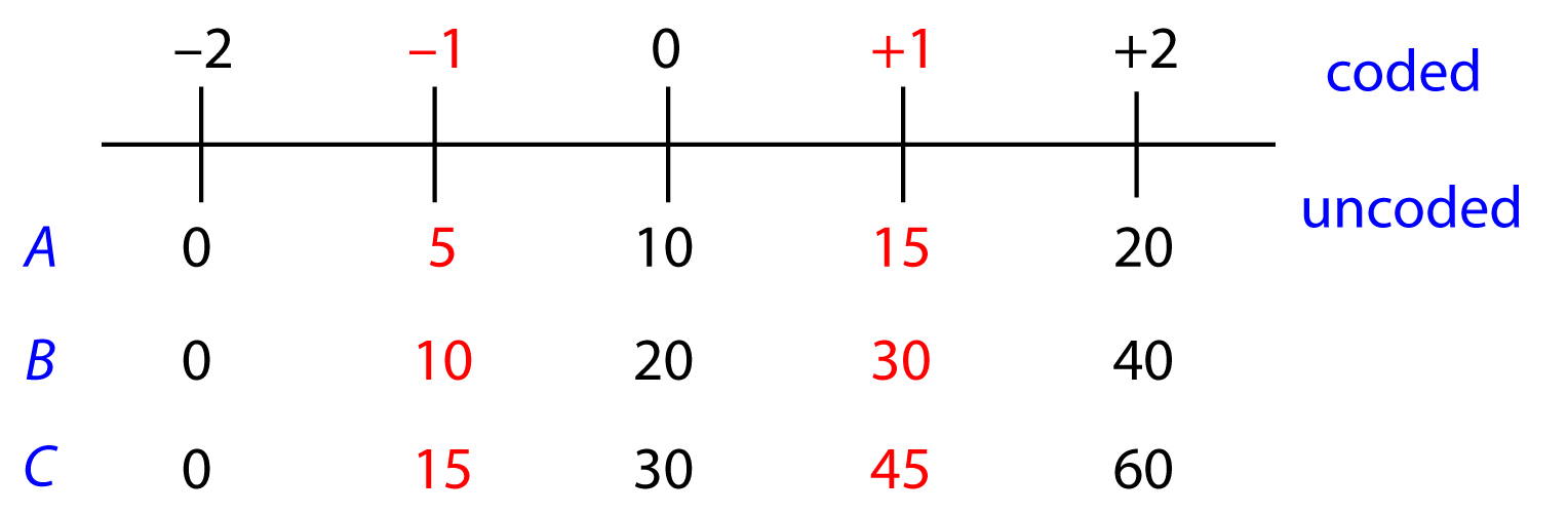
Figure 14.14 The relationship between the coded factor levels and the uncoded factor levels for Example 14.3. The numbers in red are the values defined in the 2³ factorial design.

A 2^k factorial design can model only a factor’s first-order effect on the response. A 2² factorial design, for example, includes each factor’s first-order effect (β_a and β_b) and a first-order interaction between the factors (β_ab). A 2^k factorial design cannot model higher-order effects because there is insufficient information. Here is simple example that illustrates the problem. Suppose we need to model a system in which the response is a function of a single factor. Figure 14.15a shows the result of an experiment using a 2¹ factorial design. The only empirical model we can fit to the data is a straight line.

\[R = β_0 + β_\ce{a}A\]

If the actual response is a curve instead of a straight-line, then the empirical model is in error. To see evidence of curvature we must measure the response for at least three levels for each factor. We can fit the 3¹ factorial design in Figure 14.15b to an empirical model that includes second-order factor effects.

\[R = β_0 + β_\ce{a}A+ β_\ce{aa}A^2\]

In general, an n-level factorial design can model single-factor and interaction terms up to the (n – 1)th order.

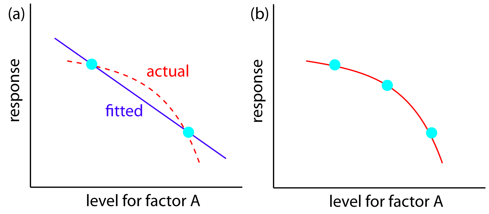
Figure 14.15 A curved one-factor response surface, in red, showing (a) the limitation of using a 2¹ factorial design, which can only fit a straight-line to the data, and (b) the application of a 3¹ factorial design that takes into account second-order effects.

We can judge the effectiveness of a first-order empirical model by measuring the response at the center of the factorial design. If there are no higher-order effects, the average response of the trials in a 2^k factorial design should equal the measured response at the center of the factorial design. To account for influence of random error we make several determinations of the response at the center of the factorial design and establish a suitable confidence interval. If the difference between the two responses is significant, then a first-order empirical model is probably inappropriate.

Note

One of the advantages of working with a coded empirical model is that b₀ is the average response of the 2 × k trials in a 2^k factorial design.

Example 14.4

One method for the quantitative analysis of vanadium is to acidify the solution by adding H₂SO₄ and oxidizing the vanadium with H₂O₂ to form a red-brown soluble compound with the general formula (VO)₂(SO₄)₃. Palasota and Deming studied the effect of the relative amounts of H₂SO₄ and H₂O₂ on the solution’s absorbance, reporting the following results for a 2² factorial design.⁵

H2SO4	H2O2	absorbance
+1	+1	0.330
+1	–1	0.359
–1	+1	0.293
–1	–1	0.420

Four replicate measurements at the center of the factorial design give absorbances of 0.334, 0.336, 0.346, and 0.323. Determine if a first-order empirical model is appropriate for this system. Use a 90% confidence interval when accounting for the effect of random error.

Solution

We begin by determining the confidence interval for the response at the center of the factorial design. The mean response is 0.335 with a standard deviation of 0.0094, which gives a 90% confidence interval of

\[=\bar X\pm \dfrac{ts}{\sqrt n}=0.335\dfrac{(2.35)(0.0094)}{\sqrt 4}=0.335\pm 0.011\]

The average response, R, from the factorial design is

\[\bar R=\dfrac{0.330+0.359+0.293+0.420}{4}=0.350\]

Because R exceeds the confidence interval’s upper limit of 0.346, we can reasonably assume that a 2² factorial design and a first-order empirical model are inappropriate for this system at the 95% confidence level.

(Problem 14.11 in the end-of-chapter problems provides a complete empirical model for this system.)

If we cannot fit a first-order empirical model to our data, we may be able to model it using a full second-order polynomial equation, such as that shown here for a two factors.

\[R = β_0 + β_\ce{a}A + β_\ce{b}B + β_\ce{aa}A^2 + β_\ce{bb}B^2 + β_\ce{ab}AB\]

Because we must measure each factor for at least three levels if we are to detect curvature (see Figure 14.15b), a convenient experimental design is a 3^k factorial design. A 3² factorial design for two factors, for example, is shown in Figure 14.16. The computations for 3^k factorial designs are not as easy to generalize as those for a 2^k factorial design and are not considered in this text. See this chapter’s additional resources for details about the calculations.

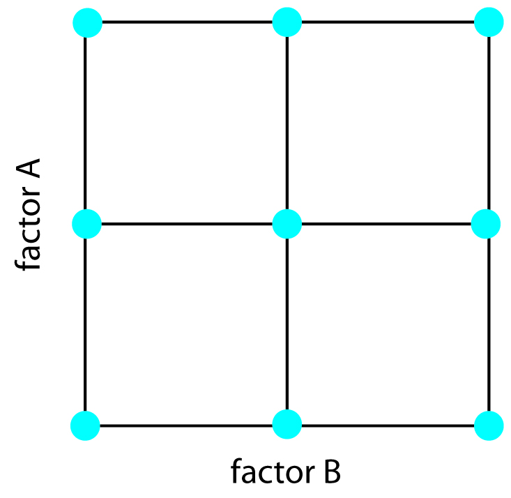
Figure 14.16 A 3^k factorial design for k = 2.

Central Composite Designs

One limitation to a 3^k factorial design is the number of trials we need to run. As shown in Figure 14.16, a 3² factorial design requires 9 trials. This number increases to 27 for three factors and to 81 for 4 factors. A more efficient experimental design for systems containing more than two factors is a central composite design, two examples of which are shown in Figure 14.17. The central composite design consists of a 2^k factorial design, which provides data for estimating each factor’s first-order effect and interactions between the factors, and a star design consisting of 2k + 1 points, which provides data for estimating second-order effects. Although a central composite design for two factors requires the same number of trials, 9, as a 3² factorial design, it requires only 15 trials and 25 trials for systems involving three factors or four factors. See this chapter’s additional resources for details about the central composite designs.

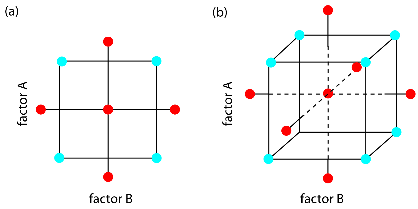
Figure 14.17 Two examples of a central composite design for (a) k = 2 and (b) k = 3. The points in blue are a 2^k factorial design, and the points in red are a star design.

Contributors

David Harvey (DePauw University)