14.6: Half-Life

Learning Objectives

• Perform calculations based on the half-life concept

Uranium isotopes produce plutonium-239 as a decay product. The plutonium can be used in nuclear weapons and is a power source for nuclear reactors, which generate electricity. This isotope has a half-life of 24,100 years, causing concern in regions where radioactive plutonium has accumulated and is stored. At some storage sites, the waste is slowly leaking into the groundwater and contaminating nearby rivers. The 24,100 year half-life means that it will be present in the earth for a very long time.

Half-Life

Radioactive materials lose some of their activity each time a decay event occurs. This loss of activity can be estimated by determining the half-life of an isotope. The half-life is defined as the period of time needed for one half of a given quantity of a substance to undergo a change. For a radioisotope, every time a decay event occurs, a count is detected on the Geiger counter, or other measuring device. A specific isotope might have a total count of \(30,000 \: \text{cpm}\). In one hour, the count could be \(15,000 \: \text{cpm}\) (half of the original count). So, the half-life of that isotope is one hour. Some isotopes have long half-lives—the half-life of \(\ce{U}\)-234 is 245,000 years. Other isotopes have shorter half-lives. \(\ce{I}\)-131, used in thyroid scans, has a half-life of 8.02 days.

Half-Life Calculations

Information on the half-life of an isotope can be used to calculate how much radioactivity of that isotope will be present after a certain period of time. There is a formula that allows calculation at any time after the initial count, but we are just going to look at loss of activity after different half-lives. The isotope \(\ce{I}\)-125 is used in certain laboratory procedures and has a half-life of 59.4 days. If the initial activity of a sample of \(\ce{I}\)-125 is \(32,000 \: \text{cpm}\), how much activity will be present in 178.2 days? Begin by determining how many half-lives are represented by 178.2 days:

\[\frac{178.2 \: \text{days}}{59.4 \: \text{days/half-life}} = 3 \: \text{half-lives}\nonumber \]

Then, simply count activity:

\[\begin{align*} \text{initial activity} \: \left( t_0 \right) &= 32,000 \: \text{cpm} \\ \text{after one half-life} \: &= 16,000 \: \text{cpm} \\ \text{after two half-lives} \: &= 8,000 \: \text{cpm} \\ \text{after three half-lives} &= 4,000 \: \text{cpm} \end{align*}\nonumber \]

Be sure to keep in mind that the initial count is at time zero \(\left( t_0 \right)\), and to subtract from that count at the first half-life. The second half-life has an activity of half the previous count (not the initial count).

For the more mathematically inclined, the following formula can be used to calculate the amount of radioactivity remaining after a given time:

\[N_t = N_0 \times \left( 0.5 \right)^\text{number of half-lives}\nonumber \]

where \(N_t =\) activity at time \(t\) and \(N_0 =\) initial activity at time \(t = 0\).

If we have an initial activity of \(42,000 \: \text{cpm}\), what will the activity be after four half-lives?

\[\begin{align*} N_t &= N_0 \left( 0.5 \right)^4 \\ &= \left( 42,000 \right) \left( 0.5 \right) \left( 0.5 \right) \left( 0.5 \right) \left( 0.5 \right) \\ &= 2625 \: \text{cpm} \end{align*}\nonumber \]

Figure \(\PageIndex{1}\): Typical radioactive decay curve.

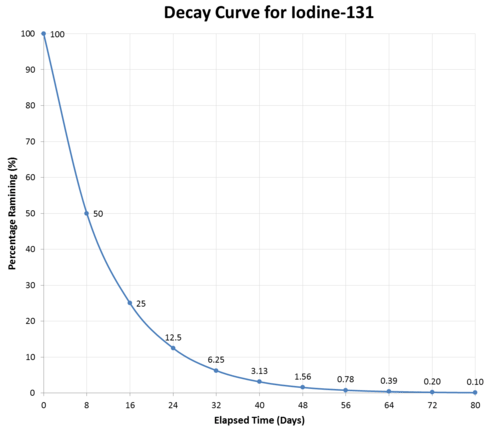
The graph above illustrates a typical decay curve for a radioactive material. The activity decreases by one-half during each succeeding half-life. Half-lives of different elements vary considerably, as shown in the table below:

Table \(\PageIndex{1}\): Isotope Half-Lives

Isotope	Decay Mode	Half-Life
Cobalt-60	beta	5.3 years
Neptunium-237	alpha	2.1 million years
Polonium-214	alpha	0.00016 seconds
Radium-224	alpha	3.7 days
Tritium (\(\ce{H}\)-3)	beta	12 years

Radioactive Decay Series

Earlier in this text, we discussed radioactive decay series. Now that we have introduced the idea of half-life, we can discuss these series in more detail. Specifically we will look at when we see a decay series, when we do not see such a decay series, and the evidence we might find that such a decay is occurring or has previously occurred.

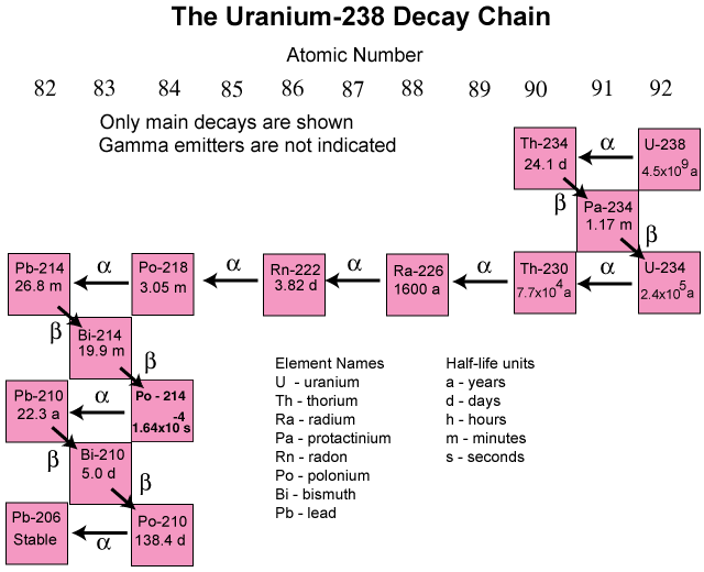
The most common is the uranium-238 decay series, which produces lead-206 in a series of 14 sequential alpha- and beta-decay reactions (Figure \(\PageIndex{2}\)). Although a radioactive decay series can be written for almost any isotope with Z > 85, only two others occur naturally: the decay of uranium-235 to lead-207 (in 11 steps) and thorium-232 to lead-208 (in 10 steps). A fourth series, the decay of neptunium-237 to bismuth-209 in 11 steps, is known to have occurred on the primitive Earth. With a half-life of “only” 2.14 million years, all the neptunium-237 present when Earth was formed decayed long ago, and today all the neptunium on Earth is synthetic.

Due to these radioactive decay series, small amounts of very unstable isotopes are found in ores that contain uranium or thorium. These rare, unstable isotopes should have decayed long ago to stable nuclei with a lower atomic number, and they would no longer be found on Earth. Because they are generated continuously by the decay of uranium or thorium, however, their amounts have reached a steady state, in which their rate of formation is equal to their rate of decay. In some cases, the abundance of the daughter isotopes can be used to date a material or identify its origin.

Figure \(\PageIndex{2}\): Decay of uranium to stable end-product.

Section Summary

• Radioactive materials lose some of their activity each time a decay event occurs.
• Radioactive loss of activity can be estimated by determining the half-life of an isotope.
• Half-life is defined as the period of time needed for one half of a given quantity of a substance to undergo a change.
• Half-lives of different elements vary considerably.