2.7.3: Ligand Group Orbitals and Generator Functions

So far we have examined the Molecular Orbital (MO) diagrams for diatomic molecules. These molecules can be classified in two different groups, those that contain hydrogen (and thus only have the hydrogen 1s orbital available to make MOs) and those that do not. For the second group, the general diagram developed in previous sections containing σ- and π-bonding and antibonding MOs will generally apply, although there can be subtle differences for heteronuclear diatomics that contain atoms with vastly different electroneagitivity values. The number of diatomic molecules is incredibly small compared to the number of molecules containing three or more atoms. It would be impractical to create and refer to general MO diagrams for all of the different possible combinations, so developing a method to quickly develop MO diagrams for these larger molecules is highly desirable. The method described will use group theory to do just that. For our purposes, we are only going to consider molecules that have a central atom surrounded by either hydrogen or a halide (which can be treated like hydrogen but with three lone pair). In other words, there will be no π-bonding in these molecules. While this again is a relatively small subset of all known molecules, it will provide a basis for the development and understanding of MO diagrams. As this course is not entirely dedicated to MO diagrams, it makes sense to take this limited approach. Larger molecules with π-bonding (and in some cases δ-bonding) requires advanced computational methods to develop MO diagrams.

The starting point to this approach is drawing a proper three-dimensional structure of the molecule of interest. From there, the point group of the molecule must be determined. Once the symmetry of the molecule is known, the symmetry of the central atom’s atomic orbitals (AOs) can be described using the appropriate symmetry labels. These are found in what is known as a character table and will be called the generator functions. The ligand group orbitals (LGOs) are then derived using a graphical approach. Combination of the generator functions and LGOs in an appropriate way gives the desired MO diagram. Using this technique, you should be able to quickly (albeit crudely) derive an MO diagram to help understand the symmetry and relative energy of the frontier orbitals, often the highest occupied molecular orbital (HOMO) and the lowest unoccupied molecular orbital (LUMO), the orbitals most responsible for chemical reactivity and spectroscopy. At this point, this approach likely seems somewhat vague at best. Rather than continue in a long narrative of the process, it is likely more effective to work through an example. This example will work through several steps that will be summarized at the end.

Step 1 - Drawing the structure and determining the hybridization of the central atom

Exercise \(\PageIndex{1}\)

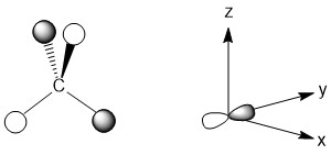
Using VSEPR, draw the three-dimensional structure of methane (CH₄).

Answer

Exercise \(\PageIndex{2}\)

What orbitals need to be used for hybridzation of the central carbon atom?

Answer

The carbon would be classified as AX₄E₀ since it is bonded to the four hydrogen atoms and has no lone pair. Based on this the carbon would have to be sp3 hybridized, which means you will need to account for the s- and all three p-orbitals on the carbon atom.

Step 2 - Determine the point group of the molecule and assign the generator functions

Exercise \(\PageIndex{3}\)

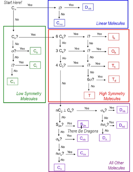
What is the point group of methane?

Answer

Methane does not have an infinite rotation axis.

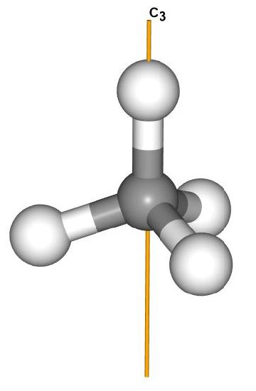
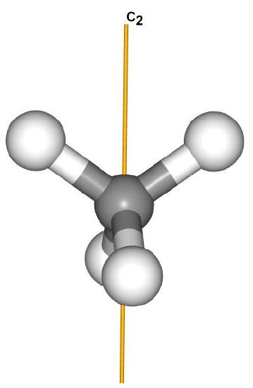
There is at least one rotation axis (in fact several). The highest order rotation axis is C₃, which can be thought of as any C-H bond. While not important for this application, there are also several C₂ axes that pass between two C-H bonds. 

There are not 6 C₅ axes.

There are not 3 C₄ axes.

There are 4 C₃ axes as each of the C-H bonds is a C₃ axis.

There is not an inversion center (it would have to be the unique carbon atom, and none of the hydrogen atoms have another hydrogen atoms directly across from it).

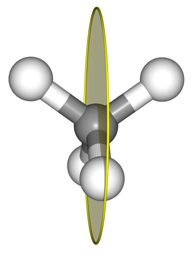
There are 6 σ.

The point group of methane is T_d.

At this point we need to turn to the character table for the point group of methane. Character tables have many uses, most of which are not applicable to this course. As such, character tables have a lot of information that will will not find necessary. Shown below are two different representations for the character table for the T_d point group. The first is the full character table while the second is an abbreviated character table that will be more useful for our purposes.

Td	E	8 C3	3 C2	6 S4	6 σd	Linear Functions	Quadratic Functions
A1	+1	+1	+1	+1	+1		x^2 + y^2 + z^2
A2	+1	+1	+1	-1	-1
E	+2	-1	+2	0	0		(2z^2-x^2-y^2, x^2-y^2)
T1	+3	0	-1	+1	-1	(Rx, Ry, Rz)
T2	+3	0	-1	-1	+1	(x, y, z)	(xy, xz, yz)

Table \(\PageIndex{1}\): Full character table for the T_d point group.

You may notice that this point group has an improper rotation (even though we did not find it when assigning the point group) and that the mirror planes are designated as σ_d. While significant and useful, there is much more information here than we need. The abbreviated character table will give us all of the information that is necessary. The table has been contracted to include on the symmetry labels (beneath T_d) and the corresponding orbitals that go with those labels. Note that some of the labels do not correspond to orbitals. The Orbitals column in the abbreviated character table corresponds to the Linear Functions column above. The (x, y, z) translates to the (p_x, p_y, p_z). The s orbital is always assigned to the row that only contains values of +1 beneath the symmetry operations. That is not significant for our purposes, but worth mentioning.

Td	Orbitals
A1	s
A2
E
T1
T2	(px, py, pz)

Table \(\PageIndex{2}\): Abbreviated character table for the T_d point group.

Exercise \(\PageIndex{4}\)

What are the symmetry labels for the orbitals on carbon used to make methane.

Answer

s - a₁

p_x - t₂

p_y - t₂

p_z - t₂

These are now our generator functions for making the LGOs. Note that the convention is a switch to lower case when assigning symmetry to orbitals.

Step 3 - Making the LGOs

Now that we have the generator functions, we can make the LGOs. This is done pictorially essentially asking the questions "What would the hydrogen 1s orbitals have to look like in order to interact in a constructive way with the carbon orbital in question?' To do this, it is very important to define the axes of your molecule before you start considering potential interactions. Due to the high symmetry of the molecule we will slightly break from convention in order to maximize orbital interactions. In group theory, the principle axis is always assigned as the z-axis, but in this case, we will assign the axes to the C₂ axes in the molecule. To begin with, let's consider the s-orbital of carbon which is labeled a₁. The s-orbital is a sphere with the same sign for the wave function in all directions (Fig. \(\PageIndex{1}\)). 

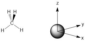
Figure \(\PageIndex{1}\): The a₁ orbital for the carbon atom in methane.

Once the axes and the orbital on carbon are drawn we want to consider what the signs for the wave functions on each hydrogen atom would have to be in order to have constructive overlap. In this case, the symmetric a₁ orbital of carbon will be able to interact with all of the hydrogen atoms in a constructive manner is they have the same sign for their wave functions (Fig. \(\PageIndex{2}\)). This generates a LGO for the hydrogen atoms that has a₁ symmetry. Although it is comprised of AOs from four hydrogen atoms, we now treat this as a single orbital for all of the hydrogen atoms hence the LGO designation.

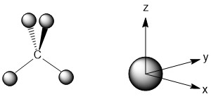
Figure \(\PageIndex{2}\): The LGO for the hydrogen atoms that has a₁​​​​​​ symmetry with the carbon generator function depicted on the axes.

The p-orbitals for the carbon atom all have the same symmetry label (t₂). One important consequence of this is that the orbitals are degenerate (equal in energy). While you would likely expect this for an isolated carbon atom, in compounds it is possible that the orbitals are no longer degenerate based on the shape of the molecule. The introduction of p-orbitals into our pictorial method adds one additional complication, p-orbitals are not symmetric and each lobe has a different sign for the wave function. In addition, p-orbitals also posses a nodal plane, a plane in which the probability of finding an electron is zero. In developing the LGO that matches with the p_z-orbital, these factors must be considered. For the p_z-orbital, the nodal plane is the xy plane. So, any hydrogen atoms that lie in the xy plane would be unable to interact with the carbon atom. That leads to an LGO that matches with the p_z-orbital as shown below (Fig. \(\PageIndex{3}\)).

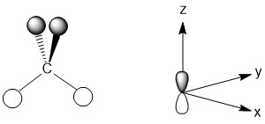
Figure \(\PageIndex{3}\): The LGO for the hydrogen atoms that has t₂​​​​​​ symmetry with the carbon generator function depicted on the axes.

None of the hydrogen atoms are in the xy plane, so they are all capable of interacting. Notice that the change in sign of the carbon p_z-orbital impacts the way the orbitals on the hydrogen atoms are represented, but does not impact the ability of those hydrogen atoms to interact.

Exercise \(\PageIndex{5}\)

Using the remaining basis functions, sketch the rest of the LGOs for the hydrogen atoms in methane.

Answer

For the p_x-orbital, the nodal plane is the yz plane. Once again none of the hydrogen atoms are in this plane so they can all interact. The LGO is depicted below. Again, the p-orbital of carbon does not point directly at any of the hydrogen atoms, but they are still capable of interacting.

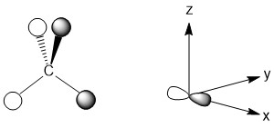
For the p_y-orbital, the nodal plane is the xz plane. Once again there are no hydrogen atoms that are unable to interact. This is a consequence of our decision to maximize the interactions possible in this highly symmetric molecule. The LGO is depicted below.

Step 4 - Constructing the MO diagram

The final step in the process is to construct the MO diagram for the molecule. Before we start constructing the MO diagram there is one final crucial question to be considered, are the atomic orbitals similar enough in energy to interact? We have actually done this to some extent already by ignoring the 1s orbital on carbon as being too low in energy to interact. Compare the energy of the valence orbitals of the atoms that are interacting and if that difference is 15 eV or less, they are close enough in energy. Like many 'rules' you have learned in chemistry, the 15 eV difference is not absolute, but is a reasonable guideline. In the case of methane, all of the orbitals are close enough in energy to interact.

Atomic Number	Element	1s	2s	2p	3s	3p	4s	4p
1	H	-13.6
2	He	-24.5
3	Li		-5.5
4	Be		-9.3
5	B		-14.0	-8.3
6	C		-19.5	-10.7
7	N		-25.5	-13.1
8	O		-32.4	-15.9
9	F		-46.4	-18.7
10	Ne		-48.5	-21.6
11	Na				-5.2
12	Mg				-7.7
13	Al				-11.3	-6.0
14	Si				-15.0	-7.8
15	P				-18.7	-10.0
16	S				-20.7	-12.0
17	Cl				-25.3	-13.7
18	Ar				-29.3	-15.9
19	K						-4.3
20	Ca						-6.1
30	Zn						-9.4
31	Ga						-12.6	-6.0
32	Ge						-15.6	-7.6
33	As						-17.6	-9.1
34	Se						-20.8	-11.0
35	Br						-24.1	-12.5
36	Kr						-27.5	-14.3

Table \(\PageIndex{3}\): Energy (eV) for valence orbitals of atoms from J.G. Verkade, A Pictorial Approach to Molecular Bonding and Vibrations, Springer-Verlag, New York, 1997, p. 69.

Building the MO diagram is similar to how it was done for diatomic molecules (Fig. \(\PageIndex{4}\)). The central atom is placed on one side and the outer atoms, as a group, are placed on the other. The relative orbital energies are approximated based on the values in Table \(\PageIndex{3}\), in this case the hydrogen LGOs fall between the a₁ and t₂ orbitals for carbon. The hydrogen LGOs are depicted as being degenerate since they are all derived from hydrogen 1s orbitals. The molecular orbitals are drawn between the carbon and hydrogen atoms. The a₁ atomic orbital on carbon has a matching a₁ LGO from hydrogen and so these orbitals can combine to give a bonding MO and an antibonding MO. As the carbon a₁ orbital is the lowest energy AO in this system it leads to the lowest energy MO. Recall that ABIMABTBIB, so it is not surprising that the lowest energy bonding orbital would give the highest energy antibonding orbital. Again, this is a rough guideline and not always the case. Dashed lines are often added to link orbitals with the same symmetry label. This is useful, but with more complex molecules can make the diagrams difficult to read. Finally, there are orbitals with t₂ symmetry on both the carbon atom and from the hydrogen LGOs. Again, these can combine to give three degenerate bonding MOs and three degenerate antibonding MOs. The exact placement of these orbitals is not critical, however, the bonding orbitals should be lower in energy than the AO and LGOs and the antibonding should be higher. The eight valence electrons are added to the system using standard electron configuration principles (Aufbau, Paulii exclusion and Hund's rule). 

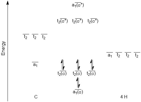
Figure \(\PageIndex{4}\): The MO diagram for CH₄.

For this system the bond order\( = \frac{8-0}{2}\ = 4\nonumber\). Notice that while this agrees with your original structure, the MO diagram shows something very different. The lowest energy bonding MO (a₁ which is depicted in c) involves all five atoms sharing two electrons, not the carbon atom and one hydrogen atom sharing. The same would be true for the bonding t₂ orbitals, more than 2 atoms are involved. In addition it would be worth noting that the HOMO would be a t₂ orbital (remember they are degenerate so a specific one can not be distinguished) and the LUMO would be a t₂ antibonding orbital.

How did we do?

Our pictorial method is qualitative but does a reasonable job of predicting the MO diagram. A more quantitative method would be to use computational methods to derive a more accurate MO diagram for this methane. The orbitals and their energies as calculated by WebMO are presented below (Table \(\PageIndex{4}\)). Overall our MO diagram looks pretty good. We see that the bonding a₁ orbital is approximately 5 eV lower in energy than the carbon a₁ orbital. The a₁* orbital is almost 40 eV higher in energy than the a₁ LGO. This is an excellent representation of the ABIMABTBIB principle. A similar trend is noted for the t₂ orbitals in which the bonding MOs are approximately 1.7 eV lower in energy than the LGOs and the t₂* orbitals are approximately 14 eV higher in energy than the carbon 2p orbitals.

(Table \(\PageIndex{4}\)). The MOs for CH₄ as calculated and displayed by WebMO. The data for CF₄ was imported into WebMO from the NIST Webbook as a computed 3-D structure and calculations were performed using B3LYP-6-31G(d). The same perspective of the molecule is used throughout.

Symmetry Label	Orbital(s)	Energy (eV)
a1*		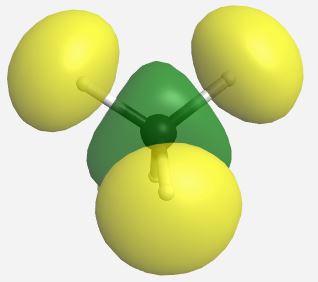26.479
t2*		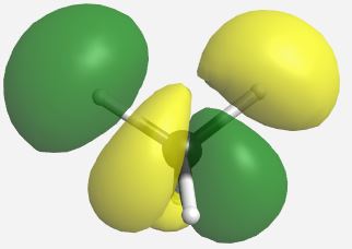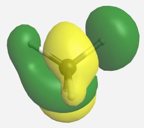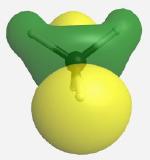3.649
t2		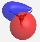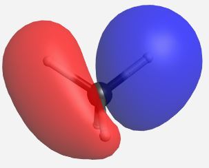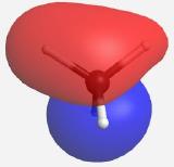-15.334
a1		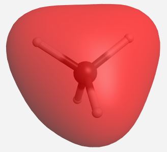-24.545

 

 Step