9.2: Crystal Field Stabilization Energy

Crystal Field Stabilization Energy

A consequence of crystal field theory is that the distribution of electrons in the d orbitals may lead to net stabilization (decrease in energy) of some complexes depending on the specific ligand geometry and metal d-electron configurations. It is a simple matter to calculate this stabilization since all that is needed is the electron configuration and knowledge of the splitting patterns.

Definition: Crystal Field Stabilization Energy (CFSE)

The crystal field stabilization energy is defined as the energy of the electron configuration in the crystal field minus the energy of the electronic configuration in the spherical field.

\[CFSE=\Delta{E}=E_{\text{crystal field}} - E_{\text{spherical field}} \label{1}\]

The CSFE will depend on multiple factors including:

• Geometry (crystal field splitting pattern)
• Number of d-electrons
• Spin Pairing Energy (the contribution of spin pairing energy is often negligible in comparison to other contributions and is omitted at times)

For an octahedral complex, each of the more stable \(t_{2g}\) orbitals are stabilized by \(-0.4\Delta_o\) relative to spherical field whereas the higher energy \(e_g\) orbitals are destabilized by \(+0.6\Delta_o\). For a complex the stabilization or destabilization of each electron is summed. Any electrons that are paired within a single orbital, also contribute spin pairing energy (+P). The overall CFSE for a complex is expressed as a multiple of the crystal field splitting parameter \(\Delta_o\).

Example \(\PageIndex{1}\): CFSE for a high Spin \(d^7\) complex

What is the CFSE for a high spin \(d^7\) octahedral complex?

Solution

The splitting pattern and electron configuration for both spherical and octahedral ligand fields are compared below.

The energy of the spherical field \((E_{\text{spherical field}}\)) is

\[ E_{\text{spherical field}}= 7 \times 0 + 2P = 2P \nonumber \]

The energy of the octahedral crystal field \(E_{\text{oct field}}\) is

\[E_{\text{oct field}} = (5 \times -0.4 \Delta_o ) + (2 \times 0.6 \Delta_o) + 2P = -0.8 \Delta_o + 2P \nonumber \]

So via Equation \ref{1}, the CFSE is

\[\begin{align} CFSE&=E_{\text{oct field}} - E_{\text{spherical field}} \nonumber \\[4pt] &=( -0.8\Delta_o + 2P ) - 2P \nonumber \\[4pt] &=-0.8 \Delta_o \nonumber \end{align} \nonumber \]

Notice that the spin pairing energy cancels out in this case (and will when calculating the CFSE of high spin complexes) since the number of paired electrons in the octahedral field is the same as that in spherical field of the free metal ion.

Exercise \(\PageIndex{1}\)

What is the CFSE for a low spin \(d^7\) octahedral complex?

Answer

The splitting pattern and electron configuration for both spherical and octahedral ligand fields are compared below.

The energy of the spherical field is the same as calculated for the high spin configuration in Example 1:

\[ E_{\text{spherical}}= 7 \times 0 + 2P = 2P \nonumber\]

The energy of the octahedral ligand\) field \(E_{\text{oct field}}\) is

\[\begin{align} E_{\text{oct field}} &= (6 \times -0.4 \Delta_o ) + (1 \times 0.6\Delta_o) + 3P \nonumber \\[4pt] &= -1.8 \Delta_o + 3P \nonumber \end{align} \nonumber \]

So via Equation \ref{1}, the CFSE is

\[\begin{align} CFSE&=E_{\text{oct field}} - E_{\text{spherical field}} \nonumber \\[4pt] &=( -9/5 \Delta_o + 3P ) - 2P \nonumber \\[4pt] &=-9/5 \Delta_o + P \nonumber \end{align} \nonumber \]

This appears more a more stable configuration than the high spin \(d^7\) configuration in Example \(\PageIndex{1}\), but we have then to take into consideration the pairing energy \(P\) to know definitely, which varies between \(200-400\; kJ\; mol^{-1}\) depending on the metal.

 

Table \(\PageIndex{1}\): Crystal field stabilization energies (CFSE) for high and low spin octahedral complexes

Total d-electrons	Spherical Field	Octahedral Field				Crystal Field Stabilization Energy
		High Spin		Low Spin
	\(E_{\text{spherical field}}\)	Configuration	\(E_{\text{crystal field}}\)	Configuration	\(E_{\text{crystal field}}\)	High Spin	Low Spin
d^0	0	\(t_{2g}^0\; e_g^0\)	0	\(t_{2g}\)^0\(e_g\)^0	0	0	0
d^1	0	\(t_{2g}^1\; e_g^0\)	-2/5 \(\Delta_o\)	\(t_{2g}\)^1\(e_g\)^0	-2/5 \(\Delta_o\)	-2/5 \(\Delta_o\)	-2/5 \(\Delta_o\)
d^2	0	\(t_{2g}^2\; e_g^0\)	-4/5 \(\Delta_o\)	\(t_{2g}\)^2\(e_g\)^0	-4/5 \(\Delta_o\)	-4/5 \(\Delta_o\)	-4/5 \(\Delta_o\)
d^3	0	\(t_{2g}^3\; e_g^0\)	-6/5 \(\Delta_o\)	\(t_{2g}\)^3\(e_g\)^0	-6/5 \(\Delta_o\)	-6/5 \(\Delta_o\)	-6/5 \(\Delta_o\)
d^4	0	\(t_{2g}^3\; e_g^1\)	-3/5 \(\Delta_o\)	\(t_{2g}\)^4\(e_g\)^0	-8/5 \(\Delta_o\) + P	-3/5 \(\Delta_o\)	-8/5 \(\Delta_o\) + P
d^5	0	\(t_{2g}^3\; e_g^2\)	0 \(\Delta_o\)	\(t_{2g}\)^5\(e_g\)^0	-10/5 \(\Delta_o\) + 2P	0 \(\Delta_o\)	-10/5 \(\Delta_o\) + 2P
d^6	P	\(t_{2g}^4\; e_g^2\)	-2/5 \(\Delta_o\) + P	\(t_{2g}\)^6\(e_g\)^0	-12/5 \(\Delta_o\) + 3P	-2/5 \(\Delta_o\)	-12/5 \(\Delta_o\) + P
d^7	2P	\(t_{2g}^5\; e_g^2\)	-4/5 \(\Delta_o\) + 2P	\(t_{2g}\)^6\(e_g\)^1	-9/5 \(\Delta_o\) + 3P	-4/5 \(\Delta_o\)	-9/5 \(\Delta_o\) + P
d^8	3P	\(t_{2g}^6\; e_g^2\)	-6/5 \(\Delta_o\) + 3P	\(t_{2g}\)^6\(e_g\)^2	-6/5 \(\Delta_o\) + 3P	-6/5 \(\Delta_o\)	-6/5 \(\Delta_o\)
d^9	4P	\(t_{2g}^6\; e_g^3\)	-3/5 \(\Delta_o\) + 4P	\(t_{2g}\)^6\(e_g\)^3	-3/5 \(\Delta_o\) + 4P	-3/5 \(\Delta_o\)	-3/5 \(\Delta_o\)
d^10	5P	\(t_{2g}^6\; e_g^4\)	0 \(\Delta_o\) + 5P	\(t_{2g}\)^6\(e_g\)^4	0 \(\Delta_o\) + 5P	0	0

\(P\) is the spin pairing energy and represents the energy required to pair up electrons within the same orbital. For a given metal ion P (pairing energy) is constant, but it does not vary with ligand and oxidation state of the metal ion).

Octahedral Preference

Similar CFSE values can be constructed for non-octahedral ligand field geometries once the knowledge of the d-orbital splitting is known and the electron configuration within those orbitals known, e.g., the tetrahedral complexes in Table \(\PageIndex{2}\). These energies geoemtries can then be contrasted to the octahedral CFSE to calculate a thermodynamic preference for a metal-ligand combination to favor the octahedral geometry. This is quantified via an octahedral site preference energy defined below.

Definition: Octahedral Site Preference Energies (OSPE)

The octahedral site preference energy (OSPE) is defined as the difference of CFSE energies for a non-octahedral complex and the octahedral complex. For comparing the preference of forming an octahedral ligand field vs. a tetrahedral ligand field, the OSPE is thus:

\[OSPE = CFSE_{(oct)} - CFSE_{(tet)} \label{2}\]

The OSPE quantifies the preference of a complex to exhibit an octahedral geometry vs. another geometry. The OSPE for octahedral vs tetrahedral geometries is illustrated below.

Note: the conversion between \(\Delta_o\) and \(\Delta_t\) used for these calculations is:

\[\Delta_t \approx \dfrac{4}{9} \Delta_o \label{3}\]

which is applicable for comparing octahedral and tetrahedral complexes that involve same ligands only.

Table \(\PageIndex{2}\): Octahedral Site Preference Energies (OSPE)

Total d-electrons	CFSE(Octahedral)		CFSE(Tetrahedral)		OSPE (for high spin complexes)**
	High Spin	Low Spin	Configuration	Always High Spin*
d^0	0 \(\Delta_o\)	0 \(\Delta_o\)	e^0	0 \(\Delta_t\)	0 \(\Delta_o\)
d^1	-2/5 \(\Delta_o\)	-2/5 \(\Delta_o\)	e^1	-3/5 \(\Delta_t\)	-6/45 \(\Delta_o\)
d^2	-4/5 \(\Delta_o\)	-4/5 \(\Delta_o\)	e^2	-6/5 \(\Delta_t\)	-12/45 \(\Delta_o\)
d^3	-6/5 \(\Delta_o\)	-6/5 \(\Delta_o\)	e^2t2^1	-4/5 \(\Delta_t\)	-38/45 \(\Delta_o\)
d^4	-3/5 \(\Delta_o\)	-8/5 \(\Delta_o\) + P	e^2t2^2	-2/5 \(\Delta_t\)	-19/45 \(\Delta_o\)
d^5	0 \(\Delta_o\)	-10/5 \(\Delta_o\) + 2P	e^2t2^3	0 \(\Delta_t\)	0 \(\Delta_o\)
d^6	-2/5 \(\Delta_o\)	-12/5 \(\Delta_o\) + P	e^3t2^3	-3/5 \(\Delta_t\)	-6/45 \(\Delta_o\)
d^7	-4/5 \(\Delta_o\)	-9/5 \(\Delta_o\) + P	e^4t2^3	-6/5 \(\Delta_t\)	-12/45 \(\Delta_o\)
d^8	-6/5 \(\Delta_o\)	-6/5 \(\Delta_o\)	e^4t2^4	-4/5 \(\Delta_t\)	-38/45 \(\Delta_o\)
d^9	-3/5 \(\Delta_o\)	-3/5 \(\Delta_o\)	e^4t2^5	-2/5 \(\Delta_t\)	-19/45 \(\Delta_o\)
d^10	0	0	e^4t2^6	0 \(\Delta_t\)	0 \(\Delta_o\)

\(P\) is the spin pairing energy and represents the energy required to pair up electrons within the same orbital.

Note

Tetrahedral complexes are always high spin since the splitting is appreciably smaller than \(P\) (Equation \ref{3}).

After conversion with Equation \ref{3}. The data in Tables \(\PageIndex{1}\) and \(\PageIndex{2}\) are represented graphically by the curves in Figure \(\PageIndex{1}\) below for the high spin complexes only. The low spin complexes require knowledge of \(P\) to graph, which will vary depending on the identiy of the metal ion.

Figure \(\PageIndex{1}\): Crystal Field Stabilization Energies for both high spin octahedral fields (\(CFSE_{oct}\)) and tetrahedral fields (\(CFSE_{tet}\)). Octahedral Site Preference Energies (OSPE) are in yellow. This is for high spin complexes only.

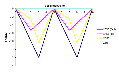
From a simple inspection of Figure \(\PageIndex{1}\), the following observations can be made:

• The OSPE is small in \(d^1\), \(d^2\), \(d^5\), \(d^6\), \(d^7\) high spin complexes and other factors influence the stability of the complexes including steric factors
• The OSPE is large in \(d^3\) and \(d^8\) high spin complexes which strongly favor octahedral geometries

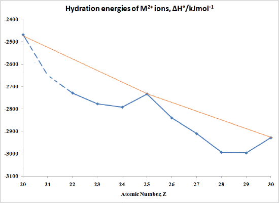
Applications

The "double-humped" curve in Figure \(\PageIndex{1}\) is found for various properties of the first-row transition metals, including hydration and lattice energies of the M(II) ions, ionic radii as well as the stability of M(II) complexes. This suggests that these properties are somehow related to crystal field effects.

In the case of hydration energies describing the complexation of water ligands to a bare metal ion:

\[M^{2+} (g) + H_2O \rightarrow [M(OH_2)_6]^{2+} (aq)\]

Table \(\PageIndex{3}\) and Figure \(\PageIndex{2}\) shows this type of curve. Note that in any series of this type not all the data are available since a number of ions are not very stable in the M(II) state in water.

Table \(\PageIndex{3}\): Hydration energies of \(M^{2+}\) ions

M	ΔH°/kJmol^-1	M	ΔH°/kJmol^-1
Ca	-2469	Fe	-2840
Sc	no stable 2+ ion	Co	-2910
Ti	-2729	Ni	-2993
V	-2777	Cu	-2996
Cr	-2792	Zn	-2928
Mn	-2733

Graphically the data in Table 2 can be represented by:

Figure \(\PageIndex{2}\): Hydration energies of \(M^{2+}\) ions

Contributors and Attributions

• Prof. Robert J. Lancashire (The Department of Chemistry, University of the West Indies)