3.7B: Homonuclear Diatomic Molecules

Introduction

Using our knowledge of how the different types of atomic orbitals can overlap and form molecular orbitals (MOs), we can now construct molecular orbital diagrams for simple diatomic molecules. In these cases we can draw and visualize all the possible ways the valence atomic orbitals on both atoms can overlap.

Creating molecular orbital diagrams

• Include all the valence atomic orbitals on both atoms, whether they are empty or filled.
• The total number of atomic orbitals MUST ALWAYS equal the total number of molecular orbitals.
• Bonding molecular orbitals are more stable than the atomic orbitals and increase the electron density between the nuclei.
• Antibonding molecular orbitals are less stable than the atomic orbitals and decrease the electron density between the nuclei.
• Fill the completed diagram with electrons according to the Aufbau principle.

First Period Diatomic Molecules

Dihydrogen (H₂)

To generate the molecular orbital diagram for H₂, begin with the valence atomic orbitals. In the case of H₂, each H atom has a single 1s valence orbital. As seen previously, then two s orbitals overlap they form a σ bonding combination and a σ* antibonding combination. The σ bonding molecular orbital increases the electron density between the two H atoms and has no nodes, which makes this combination lower in energy than the H 1s atomic orbitals. The σ* antibonding molecular orbital has a node between the two H atoms and decreases the amount of electron density between the two H atoms, which makes this combination higher energy than the H 1s atomic orbitals. This is illustrated in Figure \(\PageIndex{1}\). Notice that combining two 1s atomic orbitals has given two MOs. Each H atom has one valence electron, so two electrons are placed in the σ bonding MO.

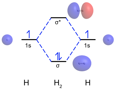 Figure \(\PageIndex{1}\): Molecular orbital diagram for H₂. Atomic and molecular orbitals calculated and visualized using WebMO. (CC BY-NC-SA; Catherine McCusker)

Bond order

Once filled with electrons, molecular orbital diagrams can be used to determine bond order in a molecule. Bond order is defined as the difference between the number of electron pairs occupying bonding and antibonding orbitals in the molecule. A bond order of 1 is equivalent to a single bond, a bond order of two is equivalent to a double bond, etc.

\[bond \,order = \frac{(bonding\, electrons)-(antibonding\, electrons)}{2}\label{bondorder}\]

Equation \ref{bondorder} can be used to calculate the bond order of a molecule from its molecular orbital diagram. In the H₂ example in Figure \(\PageIndex{1}\) There are two electrons in the sigma bonding MO and no electrons in the sigma antibonding MO. Therefore the bond order is \(\dfrac{2-0}{2} = 1\). This agrees with the picture of H₂ from the Lewis structure where the two H atoms are bonded by a single bond.

Other first period diatomics

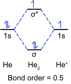
Qualitatively, the molecular orbital diagrams He₂ and any ions of H₂ and He₂ will be the same because they all will involve the overlap of two 1s atomic orbitals. What will change is the number of electrons in the diagram, and therefore the bond order. Consider the two hydrogen ions, H₂⁺ and H₂^- (Figure \(\PageIndex{2}\)). The H₂⁺ ion has one fewer electron than H₂, meaning the sigma bonding MO has one single electron in it and the sigma antibonding MO is still unoccupied. This results in H₂⁺ having a bond order of 0.5. Non-integer bond order doesn't have a direct equivalent in Lewis theory. A bond order of 0.5 tell you that the molecule is (somewhat) stable relative to the two free atoms, but the bond will be weaker than a single bond. From this we can predict that H₂⁺ will have a longer bond and a lower bond dissociation energy than H₂. H₂^- has one more electron than H₂, meaning the sigma bonding MO is filled and the additional electron occupies the sigma antibonding MO. This arrangement of electrons also results in a bond order of 0.5, so H₂^- is expected to have a bond strength and length similar to H₂⁺. In the case of He₂, each He atom has two valence electrons so the completed MO diagram has two electrons in the sigma bonding MO and 2 electrons in the sigma antibonding MO. With both the bonding an antibonding MOs completely filled, He₂ has a bond order of 0. This means that He₂ isn't energetically favorable relative to two He atoms, and should not exist. In practice, He₂ can be observed at very low temperatures, but the "bond" between the He atoms is better described as van der Waals forces than a covalent bond.

Figure \(\PageIndex{2}\): Molecular orbital diagrams for H₂⁺ (left), H₂^- (center), and He₂ (right). (CC BY-NC-SA; Catherine McCusker)

Exercise \(\PageIndex{1}\)

Draw the molecular orbital diagram for He₂⁺ and calculate its bond order.

Answer

He₂⁺ has three valence electrons, two in the sigma bonding and 1 in the sigma antibonding. This makes the bond order 0.5.

Second Period Diatomic Molecules

The four simplest molecules we have examined so far involve molecular orbitals that derived from two 1s atomic orbitals. If we wish to extend our model to larger atoms, we will have to contend with higher atomic orbitals as well. One greatly simplifying principle here is that only the valence orbitals need to be considered. Core atomic orbitals such as 1s are deep within the atom and well-shielded from the electric field of a neighboring nucleus, so that these orbitals largely retain their atomic character when bonds are formed. For second period molecules that means we need to consider the overlap of the 2s and the 2p atomic orbitals.

Dioxygen (O₂)

One major failing of Lewis and valence bond theories is their inability to explain why O₂ is paramagnetic. To construct a molecular orbital diagram for O₂ we have to consider the interactions between both the 2s and 2p atomic orbitals on each oxygen atom. Because of oxygen's high effective nuclear charge and the penetration of the 2s orbital there is a large energy difference between the 2s and the 2p atomic orbitals. This means the 2s and 2p atomic orbitals do not meet the energy criterion for overlap and cannot mix together. We will consider the overlap of the 2s and 2p orbitals separately.

The energy of the 2s atomic orbitals in oxygen are lower and the radius is larger when compared to the 1s orbitals of hydrogen, but qualitatively when two 2s orbitals overlap the will also form σ bonding and antibonding molecular orbitals as seen in Figure \(\PageIndex{3}\). As seen previously, the 2p orbitals can overlap to form both σ and π bonds. If we assume the O-O bond is on the z axis, this means the p_z orbitals on each O atom will lie along the bond axis and overlap to form σ_p bonding and σ_p* antibonding molecular orbitals. The p_x and p_y atomic orbitals both lie parallel to the bond axis and overlap to form a degenerate (same energy) pair of π_p bonding and π_p* antibonding molecular orbitals. As there is less orbital overlap in π bonds compared to σ bonds, the π_p bonding MO is stabilized less than the σ_p bonding MO and the π_p* antibonding MO is destabilized less than the σ_p* antibonding MO as shown in Figure \(\PageIndex{3}\). Each oxygen atom has six valence electrons, and so the center MO diagram is filled with 12 electrons. This leaves two electrons in the pair of π_p* antibonding MOs, and to maximize spin multiplicity according to Hund's rule one is placed in each of the MOs. Unlike the Lewis structure, the molecular orbital diagram for O₂ shows that oxygen is paramagnetic, having two unpaired electrons, in agreement with experimental observations. The MO diagram also predicts that O₂ has a bond order of 2 (\(\dfrac{8-4}{2} = 2\)) which agrees with Lewis and valence bond theories as well as experimental bond length.

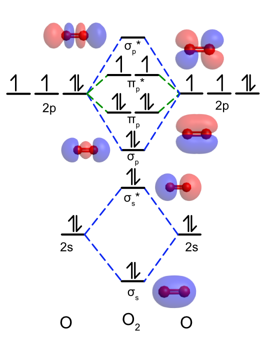
Figure \(\PageIndex{3}\): Qualitative molecular orbital diagram for O₂. Note that the energies of the atomic orbitals are not drawn to scale. Molecular orbitals calculated and visualized using WebMO. (CC BY-NC-SA; Catherine McCusker)

s-p mixing

In the molecular orbital diagram of O₂ we made the assumption that the 2s orbitals would only interact with other 2s orbitals and that 2p orbitals would only interact with other 2p orbitals because the energy difference between the 2s and 2p is large. However, in less electronegative atoms we can't make that same assumption. As Figure \(\PageIndex{4}\) illustrates, in less electronegative elements, the energies of the 2s and 2p orbitals are closer in energy and meet the energy criterion for overlap. Therefore to construct molecular orbital diagrams for most of the second period elements (except O, F, and Ne) we need to consider how the s and p orbitals can possibly overlap.

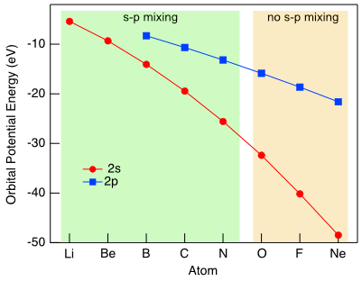
Figure \(\PageIndex{4}\): Trends in the 2s (red circle) and 2p (blue square) atomic orbital potential energies for second period elements. Energies from Meissler, G. L.; Fischer, P. J.; Tarr, D. A. Inorganic Chemistry, 5th Ed. (CC BY-NC-SA; Catherine McCusker)

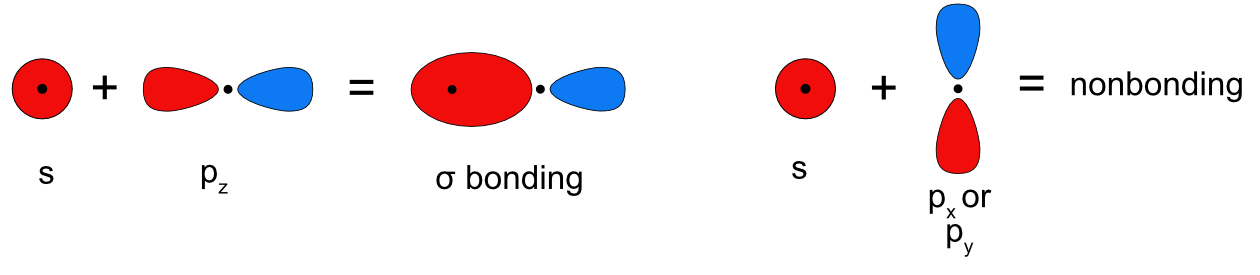
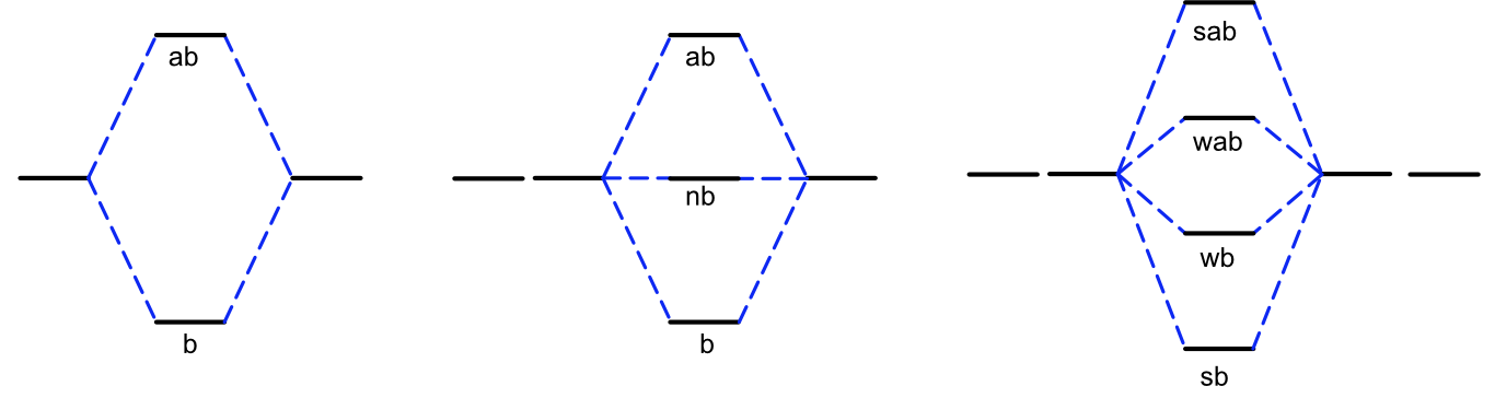
The p orbital which lies along the bond axis (p_z if we assume z is the bond axis) can overlap with the s orbital and form a sigma bonding (and antibonding) molecular orbital. The remaining two p orbitals are perpendicular to the bond axis, which means the s orbital would overlap with the node of the p orbital resulting in no net overlap and no bonding (or antibonding) MO is formed (Figure \(\PageIndex{5}\)). The s and p orbitals mixing together also means we have to consider what happens when more than two non-degenerate orbitals mix together. Based on the rules for forming molecular orbitals, the number of atomic orbitals that mix together is always equal to the number of molecular orbitals formed, as shown in Figure \(\PageIndex{6}\). When two atomic orbitals mix they form one bonding and one antibonding MO. When three atomic orbitals mix they form one bonding and one antibonding molecular orbital plus one intermediate molecular orbital that is approximately nonbonding, meaning it is neither stabilized nor destabilized relative to the atomic orbitals. When four atomic orbitals mix two bonding MOs, one strongly stabilized and one weakly stabilized, and two antibonding MOs, one strongly destabilized and one weakly destabilized, are formed.

Figure \(\PageIndex{5}\): Assuming the bond axis is the z axis, the s and p_z will overlap to form a sigma bond (left) and the s and p_x or p_y do not have the correct orientation to overlap (right). (CC BY-NC-SA; Catherine McCusker)

Figure \(\PageIndex{6}\): Two atomic orbitals (left) will overlap to form bonding (b) and antibonding (ab) molecular orbitals. Three atomic orbitals (center) will overlap to form bonding, nonbonding (nb), and antibonding molecular orbitals. Four atomic orbitals (right) will overlap to form strongly bonding (sb), weakly bonding (wb), weakly antibonding (wab) and strongly antibonding (sab) molecular orbitals. (CC BY-NC-SA; Catherine McCusker)

Dinitrogen (N₂)

Just like in O₂ the valence orbitals used to create the molecular orbital diagram of N₂ are the 2s and 2p orbitals on each N atom. Unlike the O₂ example above we cannot make the assumption that the 2s and 2p orbitals are too far apart in energy to mix together. In the case of N₂ there are four total atomic orbitals that can overlap in a sigma fashion, the 2s and 2p_z orbitals from each N atom. As shown above, when four atomic orbitals overlap the result is two bonding MOs, labeled \(\sigma_s \) and \(\sigma_s *\) in Figure \(\PageIndex{7}\) to be consistent with Figure \(\PageIndex{3}\), and two antibonding MOs, labeled \(\sigma_p \) and \(\sigma_p *\). As the 2p_x and 2p_y cannot overlap with the 2s, they form a degenerate pair of pi bonding and antibonding MOs. Each N atom has 5 valence electrons, so the N₂ molecular orbital diagram is filled with 10 total electrons, giving a bond order of 3 (\(\dfrac {8-2}{2} = 3\)). The biggest difference between the MO diagram of O₂ above and N₂ is the position of the \(\sigma_p \) MO. In O₂ it is a bonding orbital and is lower in energy than the \(\pi_p\) MOs. In N₂ this MO is weakly antibonding and is now higher than the \(\pi_p\) MOs. This change in molecular orbital ordering is the hallmark experimental observable showing s-p mixing occurs in N₂.

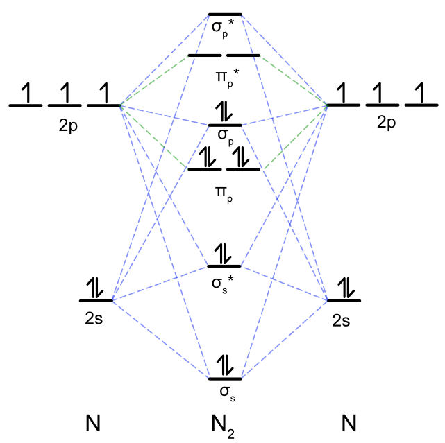
Figure \(\PageIndex{7}\): Qualitative molecular orbital diagram for N₂. Blue dashed lines indicate the mixing of 2s and 2p_z to form sigma bonding and antibonding MO's . The green dashed lines indicate the mixing of 2p_x and 2p_y to form pi bonding and antibonding MOs. Note that the energies of the atomic orbitals are not drawn to scale. (CC BY-NC-SA; Catherine McCusker)

Exercise \(\PageIndex{2}\)

Draw the complete molecular orbital diagram for B₂. Calculate the bond order and indicate whether it is diamagnetic or paramagnetic.

Answer

B₂ is paramagnetic with a bond order of 1. Bond order \(=\dfrac{4-2}{2} = 1\)

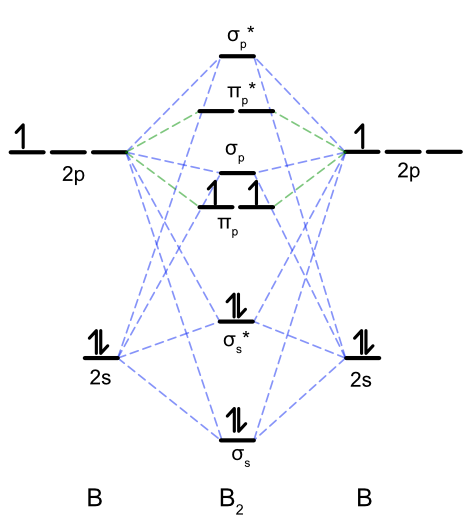
Figure for Exercise \(\PageIndex{2}\). Molecular orbital diagram of B₂. (CC-BY-NC-SA, Catherine McCusker)

Overview of Second Period Homonuclear Diatomic Molecules

Orbital mixing has significant consequences for the magnetic and spectroscopic properties of second period homonuclear diatomic molecules because it affects the order of filling of the \(\sigma(2p)\) and \(\pi(2p)\) orbitals. Early in period 2 (up to and including nitrogen), the \(\pi(2p)\) orbitals are lower in energy than the \(\sigma(2p)\) (see Figure \(\PageIndex{1})\). However, later in period 2, the \(\sigma(2p)\) orbitals are pulled to a lower energy. This lowering in energy of \(\sigma(2p)\) is not unique; all of the \(\sigma\) orbitals in the molecule are pulled to lower energy due to the increasing positive charge of the nucleus. The \(\pi\) orbitals in the molecule are also effected, but to a much lesser extent than \(\sigma\) orbitals. The reason has to do with the high penetration of s atomic orbitals compared to p atomic orbitals (recall our previous discussion on penetration and shielding, and its effect on periodic trends). The \(\sigma\) molecular orbitals have more s character and are thus their energy is more influence by increasing nuclear charge.

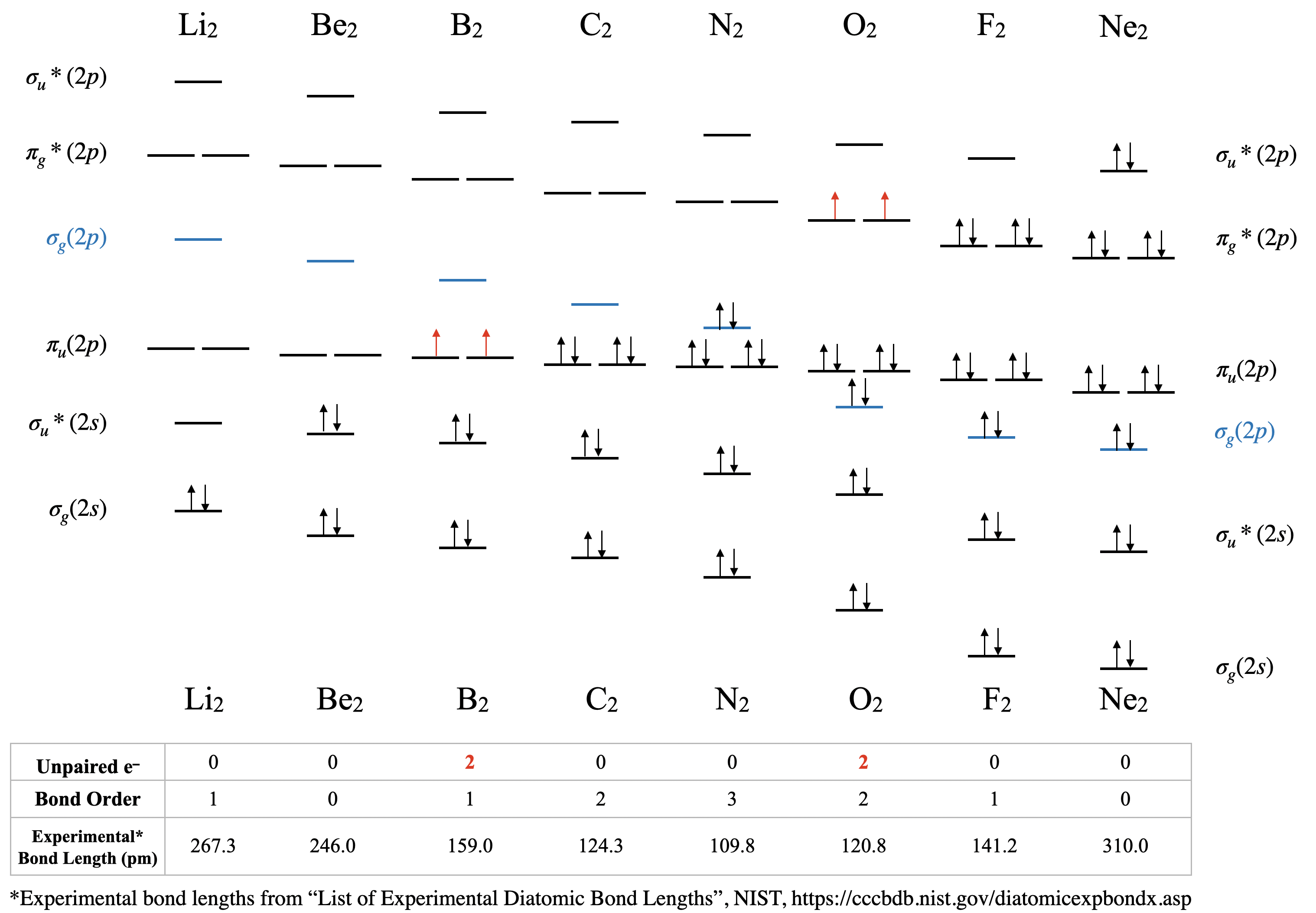
Figure \(\PageIndex{8}\): Molecular Orbital Energy-Level Diagrams for the Diatomic Molecules of the Period 2 Elements. In these diagrams, only the valence molecular orbital energy levels for the molecules are shown here (atomic orbitals not shown for simplicity). For Li₂ through N₂, the \( \sigma(2p) \) orbital is higher in energy than the \( \pi(2p) \) orbitals. In contrast, from O₂ onward, the \( \sigma(2p) \) orbital is lower in energy than the \( \pi(2p) \) orbitals due to the increase in the nuclear charge increases across the row. The experimental bond lengths correlate with calculated bond order. (CC-BY-NC-SA, Kathryn Haas)

 

Dilithium, Li₂ \([\sigma(2s)^2]\): This molecule has a bond order of one and is observed experimentally in the gas phase to have one Li-Li bond.

Diberylium, Be₂ \([\sigma(2s)^2\sigma(2s)^{*2}]\): This molecule has a bond order of zero due to equal number of electrons in bonding and antibonding orbitals. Although Be does not exist under ordinary conditions, it can be produced in a laboratory and its bond length measured (Figure \(\PageIndex{9}\)). Although the bond is very weak, its bond length is surprisingly ordinary for a covalent bond of the second period elements.

Diboron, B₂ \([\sigma(2s)^2\sigma(2s)^{*2}\pi(2p)^2]\): The case of diboron is one that is much better described by molecular orbital theory than by Lewis structures or valence bond theory. This molecule has a bond order of one. The molecular orbital description of diboron also predicts, accurately, that dibornon is paramagnetic. The paramagnetism is a consequence of sp mixing, resulting in the \(\sigma(2p)\) orbital at a higher energy than two degenerate \(\pi(2p)\) orbitals.

Dicarbon, C₂ \([\sigma(2s)^2\sigma(2s)^{*2}\pi(2p)^4]\): This molecule has a bond order of two. Molecular orbital theory predicts two bonds with \(\pi\) symmetry, and no \(\sigma\) bonding. C₂ is rare in nature because its allotrope, diamond, is much more stable.

Dinitrogen, N₂ \([\sigma(2s)^2\sigma(2s)^{*2}\pi(2p)^4\sigma(2p)^2]\): This molecule is predicted to have a triple bond. This prediction is consistent with its short bond length and bond dissociation energy. The energies of the \(\sigma(2p)\) and \(\pi(2p)\) orbitals is very close, and their relative energy levels has been a subject of some debate.

Dioxygen, O₂ \([\sigma(2s)^2\sigma(2s)^{*2}\sigma(2p)^2\pi(2p)^4\pi(2p)^{*2}]\): This is another case where valence bond theory fails to predict actual properties. Molecular orbital theory correctly predicts that dioxygen is paramagnetic, with a bond order of two. Here, the molecular orbital diagram returns to its "normal" order of orbitals where orbital mixing could be somewhat ignored, and where \(\sigma_g(2p)\) is lower in energy than \(\pi_u(2p)\).

Difluorine, F₂ \([\sigma(2s)^2\sigma(2s)^{*2}\sigma(2p)^2\pi(2p)^4\pi(2p)^{*4}]\): This molecule has a bond order of one and like oxygen, the \(\sigma(2p)\) is lower in energy than \(\pi(2p)\).

Dineon, Ne₂ \([\sigma(2s)^2\sigma(2s)^{*2}\sigma(2p)^2\pi(2p)^4\pi(2p)^{*4}\sigma(2p)^{*2}]\): Like other noble gases, Ne exists in the atomic form and does not form bonds at ordinary temperatures and pressures. Like Be₂, Ne₂ is an unstable species that has been created in extreme laboratory conditions and its bond length has been measured (Figure \(\PageIndex{9}\))

Bond Lengths

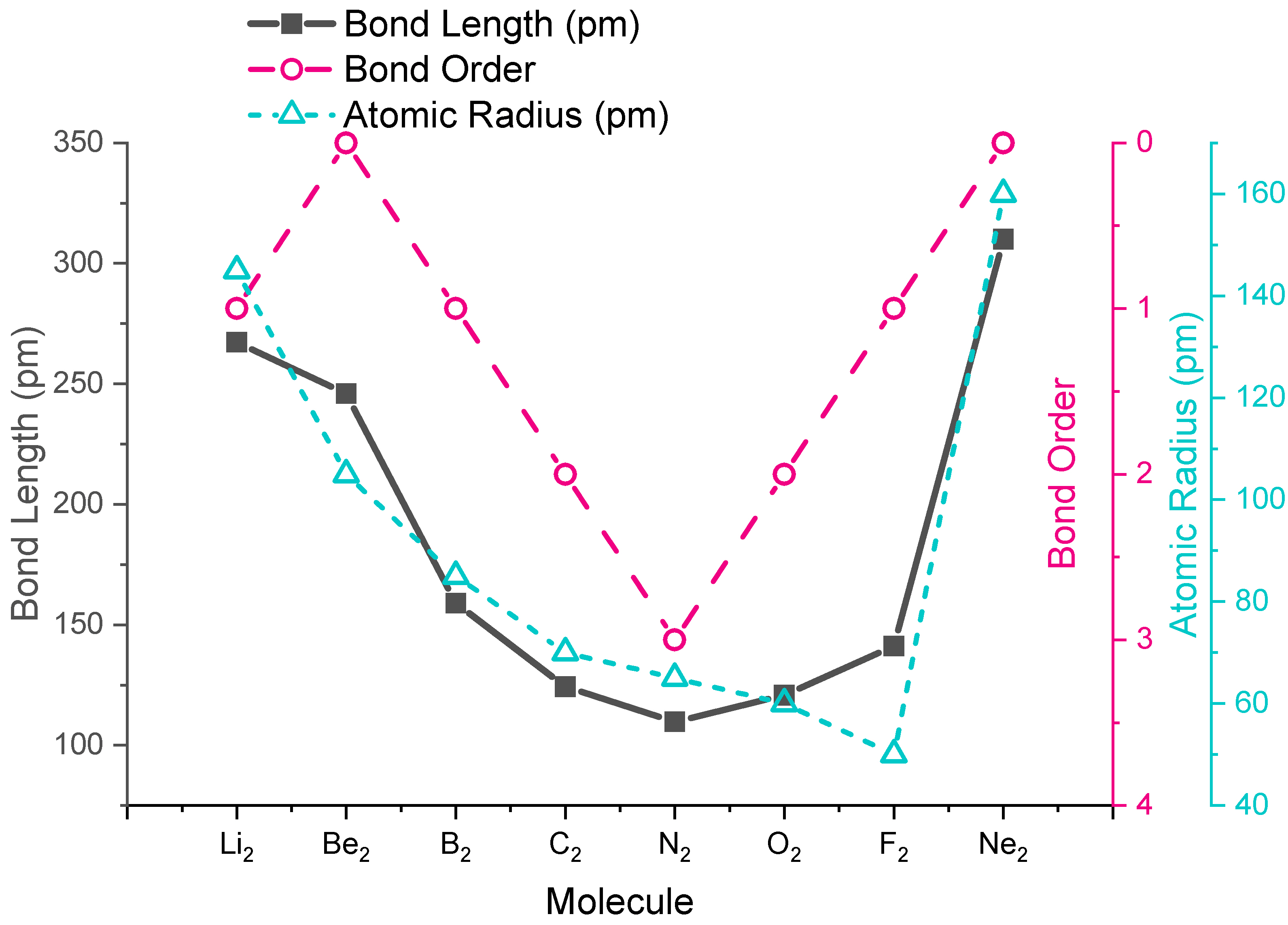
The trends in experimental bond lengths are predicted by molecular orbital theory, specifically by the calculated bond order. The values of bond order and experimental bond lengths for the second period diatomic molecules are given in Figure \(\PageIndex{8}\), and shown in graphical format on the plot in Figure \(\PageIndex{9}\). From the plot, we can see that bond length correlates well with bond order, with a minimum bond length occurring where bond order is greatest (\(\ce{N2}\)). The shortest bond distance is at \(\ce{N2}\) due to its high bond order of 3. From \(\ce{N2}\) to \(\ce{F2}\) the bond distance increases despite the fact that atomic radius decreases.

Figure \(\PageIndex{9}\): Overlayed plots of bond length (black squares), bond order (pink circles), and atomic radius (teal triangels) versus atomic number for second period homonuclear diatomic molecules. (CC-BY-NC-SA; Kathryn Haas)

References

1. Schöllkopf, W.; Toennies, J. P. Nondestructive Mass Selection of Small van der Waals Clusters. Science 1994, 266 (5189), 1345–1348.
2. NIST, Calculated Geometries available for H₂⁺ (Hydrogen cation) 2Σg+ D∞h, available at https://cccbdb.nist.gov/diatomicexpbondx.asp
3. Merritt, J. M.; Bondybey, V. E.; Heaven, M. C., Beryllium Dimer-Caught in the Act of Bonding. Science 2009, 324 (5934), 1548-1551.
4. Meissler, G. L.; Fischer, P. J.; Tarr, D. A. Inorganic Chemistry, 5th Ed; Pearson, 2014.

Contributors and Attributions

• Stephen Lower, Professor Emeritus (Simon Fraser U.) Chem1 Virtual Textbook

• Curated or created by Kathryn Haas

• Modified by Catherine McCusker, ETSU