5.8: Understanding the Value Distribution of a Variable

Last updated
Save as PDF

Page ID: 169981

\( \newcommand{\vecs}[1]{\overset { \scriptstyle \rightharpoonup} {\mathbf{#1}} } \) \( \newcommand{\vecd}[1]{\overset{-\!-\!\rightharpoonup}{\vphantom{a}\smash {#1}}} \)\(\newcommand{\id}{\mathrm{id}}\) \( \newcommand{\Span}{\mathrm{span}}\) \( \newcommand{\kernel}{\mathrm{null}\,}\) \( \newcommand{\range}{\mathrm{range}\,}\) \( \newcommand{\RealPart}{\mathrm{Re}}\) \( \newcommand{\ImaginaryPart}{\mathrm{Im}}\) \( \newcommand{\Argument}{\mathrm{Arg}}\) \( \newcommand{\norm}[1]{\| #1 \|}\) \( \newcommand{\inner}[2]{\langle #1, #2 \rangle}\) \( \newcommand{\Span}{\mathrm{span}}\) \(\newcommand{\id}{\mathrm{id}}\) \( \newcommand{\Span}{\mathrm{span}}\) \( \newcommand{\kernel}{\mathrm{null}\,}\) \( \newcommand{\range}{\mathrm{range}\,}\) \( \newcommand{\RealPart}{\mathrm{Re}}\) \( \newcommand{\ImaginaryPart}{\mathrm{Im}}\) \( \newcommand{\Argument}{\mathrm{Arg}}\) \( \newcommand{\norm}[1]{\| #1 \|}\) \( \newcommand{\inner}[2]{\langle #1, #2 \rangle}\) \( \newcommand{\Span}{\mathrm{span}}\)\(\newcommand{\AA}{\unicode[.8,0]{x212B}}\)

Discrete and Continuous Variables

Variables such as number of children in a household are called discrete variables since the possible values are discrete points on the scale. For example, a household could have three children or six children, but not 4.53 children. Other variables, such as percentage of class points earned, are continuous variables since the scale is continuous and not made up of discrete steps. The percentage could be 82.5%, or it could be 82.5149087%. Of course, the limitations of measurement, or the realities of keeping a grade book, preclude many variables from ever being truly continuous, but when measured with enough precision these variables are considered continuous for practical purposes.

Grouped Frequency Distribution for a Variable

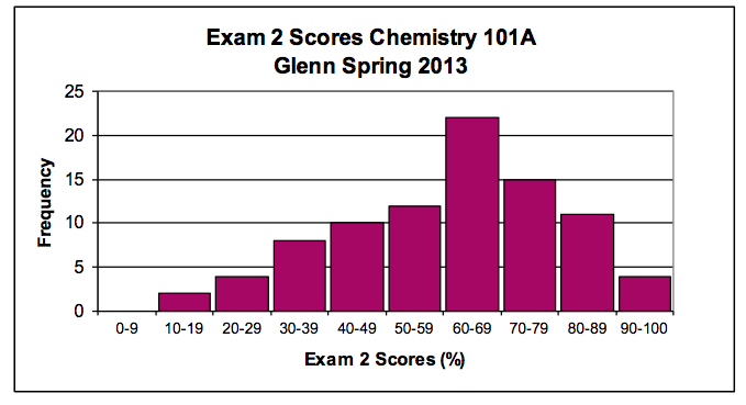
The frequency distribution for a variable consists of possible values for that variable and a count of the number of occurrences of each group of values. Consider the following grouped frequency distribution for a collection of exam scores. Typically, a grouped frequency distribution is portrayed using a histogram.

Score	0-9	10-19	20-29	30-39	40-49	50-59	60-69	70-79	80-89	90-100	*(0 -100)*
Frequency	0	2	4	8	10	12	22	15	11	4	*(88)*

grade distribution

Continuous Distribution for a Variable (Probability Density)

The histogram above portrays the actual scores from the 88 students that took this single exam in Spring 2013. However, suppose we plan to give this same exam to thousands of chemistry 101A students all throughout the state and we want to know the occurrence probability for scores between 60 and 100 percent. (That’s just another way to say we want to know what fraction of scores will be between 60 and 100 percent.) In order to accurately answer this question, we need a reasonable model for the distribution of possible values.

Mathematical equations are often used to define continuous distributions and these models are used to answer exactly this type of question. (Continuous distributions can also be called probability densities.) The normal distribution or “bell curve” is, perhaps, the best known example of a continuous distribution. Many empirical distributions are approximated well by mathematical distributions such as the normal distribution. An example of a normal distribution is shown below. Many exam score distributions are modeled using a similar curve.

Normal curve

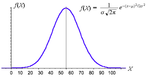
The y-axis in the distribution technically represents the “fraction per unit” or the "probability density." You do not use the actual y-axis values very often and no y-values are shown in the image above. Intuitively, the y-axis value tells you the chance of obtaining values near corresponding points on the x-axis. In the normal distribution pictured, the probability of an observation with a value near 40 is about half of the probability of an observation with value near 50. The most probable value is the value of x corresponding to the highest value of y (the “peak” of the curve.) In the normal distribution pictured, 55 the most probable value of x.

Although we will not discuss the concept of a continuous distribution in great detail, you must be familiar with the following ideas:

1) The fraction of sample values equal to an exact single value of x is a very small number! Consider our exam score example. What fraction of exams will have a score equal to exactly 82.31 percent? That’s a ridiculously specific score! So, it should make sense that the fraction of exams that have that score is going to be a very, very, very small number. The fraction of exams that will have a score equal to exactly 82.31956432342346576 percent is essentially zero. (We can make the fraction as close as we like to zero by making the exam score more and more precise.)

2) Continuous distributions are best used to determine the fraction of sample with values within a range of x values. Again, consider the exam score example. What fraction of exams will have a score between 80 and 90 percent? That will be a significant portion of the sample and we would expect that the fraction of exams with scores within that range will be much larger than the fraction for a single score (as described above.)

3) The fraction of area under the curve in any particular region tells you the fraction of the sample with values within that range. For a normalized distribution, the total area under the curve equals 1. Suppose that one tenth of the exam scores are between 80 and 90 percent. This can be seen in the distribution plot! The continuous distribution for the scores would have a shape that places one tenth of the area below the curve in the region bounded by 80 and 90 on the x-axis.