Section 6.1: Crystal Field Theory

Crystal Field Theory

Crystal field theory (CFT) describes the breaking of orbital degeneracy in transition metal complexes due to the presence of ligands. CFT qualitatively describes the strength of the metal-ligand bonds. Based on the strength of the metal-ligand bonds, the energy of the system is altered. This may lead to a change in magnetic properties as well as color. This theory was developed by Hans Bethe and John Hasbrouck van Vleck in the late 1920's. Crystal field theory is a purely electrostatic theory and uses classical potential energy equations that take into account the attractive and repulsive interactions between charged particles (that is, Coulomb's Law interactions).

\[E \propto \dfrac{q_1 q_2}{r}\]

with

• \(E\) the bond energy between the charges and
• \(q_1\) and \(q_2\) are the charges of the interacting ions and
• \(r\) is the distance separating them.

For this simple approach to work, CFT makes some assumptions and simplifications. All ligands are modeled as negative point charges with no orbitals and the metal orbitals are modeled as clouds of negative charge. This approach leads to the correct prediction that large cations of low charge, such as \(K^+\) and \(Na^+\), should form few coordination compounds. For transition metal cations that contain varying numbers of d electrons in orbitals that are NOT spherically symmetric, however, the situation is quite different. The shape and occupation of these d-orbitals then becomes important in an accurate description of the bond energy and properties of the transition metal compound.

Orientation of d-Orbitals

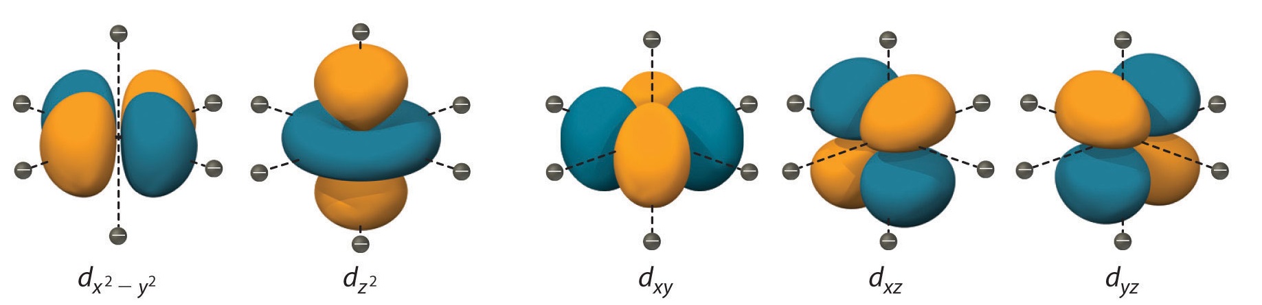
To understand CFT, one must first understand the shape and orientation of the d orbitals:

• d_xy: lobes lie in-between the x and the y axes.
• d_xz: lobes lie in-between the x and the z axes.
• d_yz: lobes lie in-between the y and the z axes.
• d_x²-y²: lobes lie on the x and y axes.
• d_z²: there are two lobes on the z axes and there is a donut shape ring that lies on the xy plane around the other two lobes.

Figure \(\PageIndex{1}\): Spatial arrangement of ligands in the an octahedral ligand field with respect to the five d-orbitals.

Octahedral Crystal Field

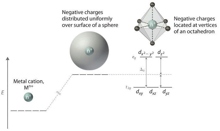
When examining a single transition metal ion in free space, the five d-orbitals have the same energy (Figure \(\PageIndex{2}\)). When ligands approach the metal ion, the ligand negative point charges destabilize the metal d-orbital based on the geometric structure of the molecule. Since ligands approach from different directions, not all d-orbitals interact equally. These interactions, however, create a splitting due to the electrostatic environment, orbitals with more interaction are higher in energy and orbitals with less interaction are lower in energy.

Definition: Barycenter

In crystal field theory the barycenter is the energy of the d orbitals in a spherical crystal field, where the negative lignad charges are evenly distributed around the metal ion in a sphere. The splitting of the d orbitals in other crystal fields will be symmetric around the barycenter (i.e. the total amount of stabalization will always be equal to the total amount of destabalization)

For example, consider a molecule with octahedral geometry. Ligands approach the metal ion along the \(x\), \(y\), and \(z\) axes. Therefore, the electrons in the \(d_{z^2}\) and \(d_{x^2-y^2}\) orbitals (which lie along these axes) experience greater repulsion and are therefore at higher energy. Compared to a spherical field, where ligands are evenly distributed around the metal center, the d orbitals that lie between the axes (\(d_{xy}\), \(d_{xz}\), and \(d_{yz}\) experience less repulsion when the ligands are in an octahedral arrangement and are stabilized. This causes a splitting in the energy levels of the d-orbitals, known as crystal field splitting. For octahedral complexes, crystal field splitting is denoted by \(\Delta_o\) (or \(\Delta_{oct}\)) (in older texts and papers it may also be labeled as 10Dq). Any orbital that has a lobe on the axes moves to a higher energy level. The energies of the e_g symmetry orbitals (\(d_{z^2}\) and \(d_{x^2-y^2}\)) increase due to greater interactions with the ligands. The t_2g symmetry orbitals (\(d_{xy}\), \(d_{xz}\), and \(d_{yz}\)) decrease in energy with respect to the spherical energy level and become more stable. This splitting is symmetric around the barycenter (the theoretical energy of the d orbitals with spherical charge distribution) which means that the energy levels of e_g are higher (by 0.6∆_o) while t_2g are lower (by 0.4∆_o). It should be noted that the labels t_2g and e_g come from group theory and the octahedral point group. The energy difference between the t_2g and e_g orbitals dictates the energy that the complex will absorb causing electrons to move from one level to the next. For transition metal complexes, the absorbed energy is typically in the visible part of the spectrum and thus this will determine the color of the complex. Whether the complex is paramagnetic or diamagnetic will be determined by the spin state. If there are unpaired electrons, the complex is paramagnetic; if all electrons are paired, the complex is diamagnetic.

Figure \(\PageIndex{2}\): (a) Distributing a charge of −6 uniformly over a spherical surface surrounding a metal ion causes the energy of all five d orbitals to increase due to electrostatic repulsions, but the five d orbitals remain degenerate. Placing a charge of −1 at each vertex of an octahedron causes the d orbitals to split into two groups with different energies: the d_x²−y² and d_z² orbitals increase in energy, while the, d_xy, d_xz, and d_yz orbitals decrease in energy. The average energy of the five d orbitals is the same as for a spherical distribution of a −6 charge, however. Attractive electrostatic interactions between the negatively charged ligands and the positively charged metal ion (far right) cause all five d orbitals to decrease in energy but does not affect the splittings of the orbitals. (b) The two e_g orbitals (left) point directly at the six negatively charged ligands, which increases their energy compared with a spherical distribution of negative charge. In contrast, the three t_2g orbitals (right) point between the negatively charged ligands, which decreases their energy compared with a spherical distribution of charge.

Filling Electrons in Orbitals

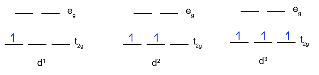
d¹ - d³

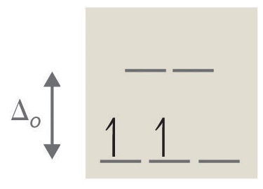
For one, two, or three d electrons the filling is straightforward. According to the Aufbau principle, electrons are filled from lower to higher energy orbitals. In an octahedral crystal field, this corresponds to the \(d_{xy}\), \(d_{xz}\), and \(d_{yz}\)) orbitals. Following Hund's rule, electrons are filled in order to have the highest number of unpaired electrons. Therefore, each electron occupies one of the t_2g symmetry orbitals \(d_{xy}\), \(d_{xz}\), or \(d_{yz}\)) and all the electrons are orientated in the same direction to maximize spin multiplicity as shown in Figure \(\PageIndex{3}\).

Figure \(\PageIndex{3}\): Arrangement of the d electrons in a octahedral crystal field for 1, 2, and 3 d electrons. (CC-BY-NC-SA; Catherine McCusker)

d⁴ - d⁷

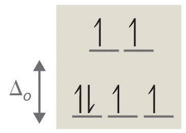
When a complex has between 4 and 7 d electrons there are two ways the electrons can be arranged into the d orbitals. As an example, in d⁴ the first three electrons are placed one in each of the t_2g symmetry orbitals. The fourth electron can either be placed in one of the empty e_g symmetry orbitals or it can be paired in one or the t_2g symmetry orbitals, as shown in Figure \(\PageIndex{4}\). The first configuration is called high spin because it maximizes the number of unpaired electrons and the second is called low spin. Whether a complex will have the high spin or low configuration depends on the relative magnitude of the spin pairing energy (the energy required to place two negatively charged electrons in the same orbital) and the crystal field splitting (\(\Delta_o\)). In cases where the spin pairing energy is larger than \(\Delta_o\) the complex will adopt the high spin configuration because it requires less energy to place an electron in a higher energy e_g orbital than is does to pair two electrons in the same t_2g orbital. In cases where \(\Delta_o\) is larger than the spin pairing energy the complex will adopt a low spin configuration because it requires less energy to place a second electron in a t_2g orbital than it does to place one in the higher energy e_g orbitals.

Definition: Spin Pairing Energy

The spin pairing energy is the energy required to pair two electrons in an orbital. It is based on the Coulombic repulsion between the two negative charges. Larger, more diffuse orbitals will have lower spin pairing energy because the two electrons can be further apart

Figure \(\PageIndex{4}\): High spin and low spin arrangements of electrons for d⁴ - d⁷. (CC-BY-NC-SA; Catherine McCusker)

d⁸ - d¹⁰

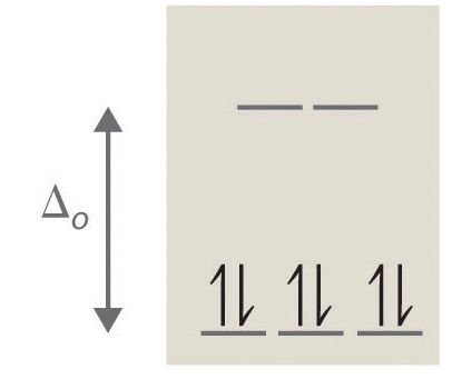
For complexes with 8 - 10 d electrons there is again only one way to arrange the electrons. Whether or not the e_g orbitals are filled before electrons are paired in the t_2g orbitals the final electron configurations are as shown in Figure \(\PageIndex{5}\).

Figure \(\PageIndex{5}\): Arrangement of the d electrons in a octahedral crystal field for 8, 9, and 10 d electrons. (CC-BY-NC-SA; Catherine McCusker)

Tetrahedral Crystal Field

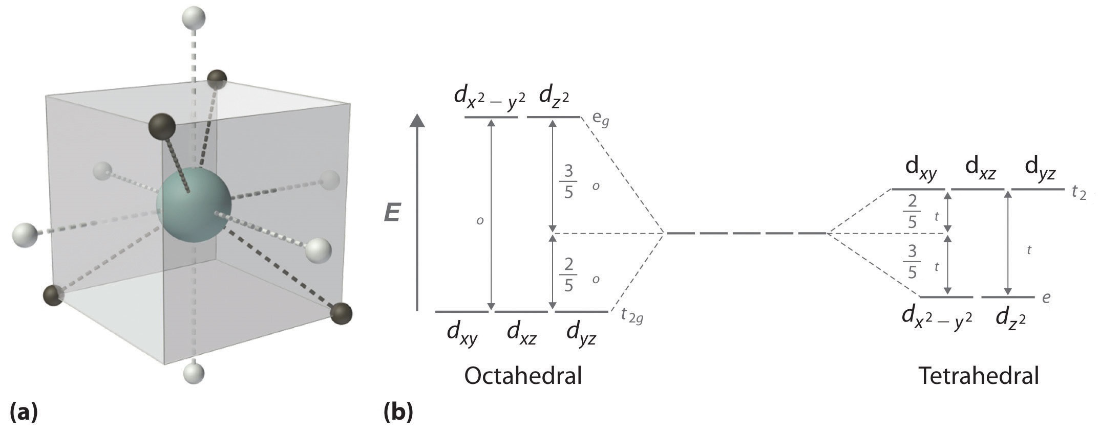
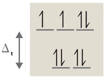
In a tetrahedral complex, the four ligands are orientated at opposite corners of a cube as shown in Figure \(\PageIndex{6a}\) rather than along the axes. With the ligands between the axes, the three d orbitals which lie between the axes, \(d_{xy}\), \(d_{xz}\), and \(d_{yz}\) (t₂ symmetry in tetrahedral), now interact more with the ligands and are destabilized relative to the spherical crystal field. Conversely, the two d orbitals that lie along the axes, \(d_{x^2-y^2}\) and \(d_{z^2}\) (e symmetry in tetrahedral), now interact less with the d orbitals and are stabilized relative to the spherical crystal field. As shown in Figure \(\PageIndex{6b}\) the splitting of the d orbitals in a tetrahedral crystal field is essentially the inverse of the octahedral crystal field. The crystal field splitting energy in a tetrahedral crystal field is \(\Delta_{t}\). Because a tetrahedral complex has fewer ligands than an octahedral complex, and those ligands are not ideally orientated to overlap with the d orbitals \(\Delta_{t}\) is less than \(\Delta_{o}\) for the same metal and ligands:

\[\Delta_{t} \approx \frac{4}{9}\,\Delta_o \label{1}\]

Consequentially, \(\Delta_{t}\) is typically smaller than the spin pairing energy, so tetrahedral complexes are usually high spin. As seen with octahedral compounds, the labels for the groups of orbitals, t₂ and e in this case, come from group theory and the tetrahedral point group.

Figure \(\PageIndex{6}\): (a) Tetrahedral ligand field surrounding a central transition metal (teal sphere). (b) Splitting of the degenerate d-orbitals (without a ligand field) due to an octahedral ligand field (left diagram) and the tetrahedral field (right diagram).

Square Planar Crystal Field

In a complex with four ligands, the other possible arrangement of ligands is square planar. The easiest way to visualize the square planar geometry is to start with an octahedral complex and remove the two ligands that are along the z axis. The four remaining ligands are in the xy plane, along the x and y axes. From a crystal field splitting perspective, when the z ligands are removed the d orbitals split further. In an octahedral crystal field both \(d_{x^2-y^2}\) and \(d_{z^2}\) are destabilized. When the z ligands are removed the \(d_{z^2}\) orbital is stabilized because it no longer interacts with ligands on the z axis. Conversely the \(d_{x^2-y^2}\) orbital is further destabilized because all of the ligand negative charges are concentrated in the xy plane. Removing the z ligand has a similar effect on the \(d_{xy}\), \(d_{xz}\), and \(d_{yz}\) orbitals, although the magnitude of the stabilization and destabilization is less because those orbitals do not directly interact with the ligands. The \(d_{xy}\) orbital is destabilized because it also lies in the xy plane and the \(d_{xz}\) and \(d_{yz}\) orbitals are stabilized because they have lost the (indirect) interaction with the ligands on the z axis. Overall the \(d_{x^2-y^2}\) orbital is significantly more destabilized than the other d orbitals, meaning the square planar geometry is most favored in complexes with 8 electrons where the \(d_{x^2-y^2}\) is empty and the other more stabilized d orbitals are filled.

Figure \(\PageIndex{7}\): Comparison between octahedral and square planar crystal field splittings, showing how the energies of the d orbitals change when the two z ligands are removed from an octahedral complex to form a square planar complex. (CC-BY-NC-SA; Catherine McCusker)

Video:

Tetrahedral vs Square Planar

From VSEPR theory we know that sterically the most favorable way to arrange four ligands around a metal ion is in the tetrahedral arrangement. That puts the most possible space between the four ligands. Because of this, a four coordinate metal complex will prefer a tetrahedral geometry UNLESS there is a larger crystal field stabilization energy (CFSE) for the square planar arrangement. As discussed above, this means square planar is the preferred geometry for most metal complexes with 8 d electrons, especially when the crystal field splitting (Δ) is large. While not every d⁸ complex is square planar, almost all square planar complexes are d⁸ (there are examples of d⁷ and d⁹ square planar complexes but they are less common)

Exercise \(\PageIndex{3}\)

For each of the following, sketch the d-orbital splitting diagram, fill the diagram with the correct number of d-electrons, list the number of unpaired electrons, and label whether they are paramagnetic or diamagnetic:

1. [Ti(H₂O)₆]²⁺
2. [NiCl₄]^2- (tetrahedral)
3. [CoF₆]^3- (high spin)
4. [Co(NH₃)₆]³⁺ (low spin)

Answer

1. 2 unpaired electrons, paramagnetic

2. 2 unpaired electrons, paramagnetic

3. 4 unpaired electrons, paramagnetic

4. 0 unpaired electrons, diamagnetic

Contributors and Attributions

• Asadullah Awan (UCD), Hong Truong (UCD)

• Prof. Robert J. Lancashire (The Department of Chemistry, University of the West Indies)

• Modified by Catherine McCusker (East Tennessee State University)