
6.10: Using Excel and R to Solve Equilibrium Problems
- Page ID
- 220707

\( \newcommand{\vecs}[1]{\overset { \scriptstyle \rightharpoonup} {\mathbf{#1}} } \)
\( \newcommand{\vecd}[1]{\overset{-\!-\!\rightharpoonup}{\vphantom{a}\smash {#1}}} \)
\( \newcommand{\id}{\mathrm{id}}\) \( \newcommand{\Span}{\mathrm{span}}\)
( \newcommand{\kernel}{\mathrm{null}\,}\) \( \newcommand{\range}{\mathrm{range}\,}\)
\( \newcommand{\RealPart}{\mathrm{Re}}\) \( \newcommand{\ImaginaryPart}{\mathrm{Im}}\)
\( \newcommand{\Argument}{\mathrm{Arg}}\) \( \newcommand{\norm}[1]{\| #1 \|}\)
\( \newcommand{\inner}[2]{\langle #1, #2 \rangle}\)
\( \newcommand{\Span}{\mathrm{span}}\)
\( \newcommand{\id}{\mathrm{id}}\)
\( \newcommand{\Span}{\mathrm{span}}\)
\( \newcommand{\kernel}{\mathrm{null}\,}\)
\( \newcommand{\range}{\mathrm{range}\,}\)
\( \newcommand{\RealPart}{\mathrm{Re}}\)
\( \newcommand{\ImaginaryPart}{\mathrm{Im}}\)
\( \newcommand{\Argument}{\mathrm{Arg}}\)
\( \newcommand{\norm}[1]{\| #1 \|}\)
\( \newcommand{\inner}[2]{\langle #1, #2 \rangle}\)
\( \newcommand{\Span}{\mathrm{span}}\) \( \newcommand{\AA}{\unicode[.8,0]{x212B}}\)
\( \newcommand{\vectorA}[1]{\vec{#1}} % arrow\)
\( \newcommand{\vectorAt}[1]{\vec{\text{#1}}} % arrow\)
\( \newcommand{\vectorB}[1]{\overset { \scriptstyle \rightharpoonup} {\mathbf{#1}} } \)
\( \newcommand{\vectorC}[1]{\textbf{#1}} \)
\( \newcommand{\vectorD}[1]{\overrightarrow{#1}} \)
\( \newcommand{\vectorDt}[1]{\overrightarrow{\text{#1}}} \)
\( \newcommand{\vectE}[1]{\overset{-\!-\!\rightharpoonup}{\vphantom{a}\smash{\mathbf {#1}}}} \)
\( \newcommand{\vecs}[1]{\overset { \scriptstyle \rightharpoonup} {\mathbf{#1}} } \)
\( \newcommand{\vecd}[1]{\overset{-\!-\!\rightharpoonup}{\vphantom{a}\smash {#1}}} \)
\(\newcommand{\avec}{\mathbf a}\) \(\newcommand{\bvec}{\mathbf b}\) \(\newcommand{\cvec}{\mathbf c}\) \(\newcommand{\dvec}{\mathbf d}\) \(\newcommand{\dtil}{\widetilde{\mathbf d}}\) \(\newcommand{\evec}{\mathbf e}\) \(\newcommand{\fvec}{\mathbf f}\) \(\newcommand{\nvec}{\mathbf n}\) \(\newcommand{\pvec}{\mathbf p}\) \(\newcommand{\qvec}{\mathbf q}\) \(\newcommand{\svec}{\mathbf s}\) \(\newcommand{\tvec}{\mathbf t}\) \(\newcommand{\uvec}{\mathbf u}\) \(\newcommand{\vvec}{\mathbf v}\) \(\newcommand{\wvec}{\mathbf w}\) \(\newcommand{\xvec}{\mathbf x}\) \(\newcommand{\yvec}{\mathbf y}\) \(\newcommand{\zvec}{\mathbf z}\) \(\newcommand{\rvec}{\mathbf r}\) \(\newcommand{\mvec}{\mathbf m}\) \(\newcommand{\zerovec}{\mathbf 0}\) \(\newcommand{\onevec}{\mathbf 1}\) \(\newcommand{\real}{\mathbb R}\) \(\newcommand{\twovec}[2]{\left[\begin{array}{r}#1 \\ #2 \end{array}\right]}\) \(\newcommand{\ctwovec}[2]{\left[\begin{array}{c}#1 \\ #2 \end{array}\right]}\) \(\newcommand{\threevec}[3]{\left[\begin{array}{r}#1 \\ #2 \\ #3 \end{array}\right]}\) \(\newcommand{\cthreevec}[3]{\left[\begin{array}{c}#1 \\ #2 \\ #3 \end{array}\right]}\) \(\newcommand{\fourvec}[4]{\left[\begin{array}{r}#1 \\ #2 \\ #3 \\ #4 \end{array}\right]}\) \(\newcommand{\cfourvec}[4]{\left[\begin{array}{c}#1 \\ #2 \\ #3 \\ #4 \end{array}\right]}\) \(\newcommand{\fivevec}[5]{\left[\begin{array}{r}#1 \\ #2 \\ #3 \\ #4 \\ #5 \\ \end{array}\right]}\) \(\newcommand{\cfivevec}[5]{\left[\begin{array}{c}#1 \\ #2 \\ #3 \\ #4 \\ #5 \\ \end{array}\right]}\) \(\newcommand{\mattwo}[4]{\left[\begin{array}{rr}#1 \amp #2 \\ #3 \amp #4 \\ \end{array}\right]}\) \(\newcommand{\laspan}[1]{\text{Span}\{#1\}}\) \(\newcommand{\bcal}{\cal B}\) \(\newcommand{\ccal}{\cal C}\) \(\newcommand{\scal}{\cal S}\) \(\newcommand{\wcal}{\cal W}\) \(\newcommand{\ecal}{\cal E}\) \(\newcommand{\coords}[2]{\left\{#1\right\}_{#2}}\) \(\newcommand{\gray}[1]{\color{gray}{#1}}\) \(\newcommand{\lgray}[1]{\color{lightgray}{#1}}\) \(\newcommand{\rank}{\operatorname{rank}}\) \(\newcommand{\row}{\text{Row}}\) \(\newcommand{\col}{\text{Col}}\) \(\renewcommand{\row}{\text{Row}}\) \(\newcommand{\nul}{\text{Nul}}\) \(\newcommand{\var}{\text{Var}}\) \(\newcommand{\corr}{\text{corr}}\) \(\newcommand{\len}[1]{\left|#1\right|}\) \(\newcommand{\bbar}{\overline{\bvec}}\) \(\newcommand{\bhat}{\widehat{\bvec}}\) \(\newcommand{\bperp}{\bvec^\perp}\) \(\newcommand{\xhat}{\widehat{\xvec}}\) \(\newcommand{\vhat}{\widehat{\vvec}}\) \(\newcommand{\uhat}{\widehat{\uvec}}\) \(\newcommand{\what}{\widehat{\wvec}}\) \(\newcommand{\Sighat}{\widehat{\Sigma}}\) \(\newcommand{\lt}{<}\) \(\newcommand{\gt}{>}\) \(\newcommand{\amp}{&}\) \(\definecolor{fillinmathshade}{gray}{0.9}\)In solving equilibrium problems we typically make one or more assumptions to simplify the algebra. These assumptions are important because they allow us to reduce the problem to an equation in x that we can solve by simply taking a square‐root, a cube‐root, or by using the quadratic equation. Without these assumptions, most equilibrium problems result in a cubic equation (or a higher‐order equation) that is more challenging to solve. Both Excel and R are useful tools for solving such equations.
Although we focus here on the use of Excel and R to solve equilibrium problems, you also can use WolframAlpha; for details, see Cleary, D. A. “Use of WolframAlpha in Equilibrium Calculations,” Chem. Educator, 2014, 19, 182–186.
Excel
Excel offers a useful tool—the Solver function—for finding the chemically significant root of a polynomial equation. In addition, it is easy to solve a system of simultaneous equations by constructing a spreadsheet that allows you to test and evaluate multiple solutions. Let’s work through two examples.
Example 1: Solubility of Pb(IO3)2 in 0.10 M Pb(NO3)2
In our earlier treatment of this problem we arrived at the following cubic equation
\[4 x^{3}+0.40 x^{2}=2.5 \times 10^{-13} \nonumber\]
where x is the equilibrium concentration of Pb2+. Although there are several approaches for solving cubic equations with paper and pencil, none are computationally easy. One approach is to iterate in on the answer by finding two values of x, one that leads to a result larger than \(2.5 \times 10^{-13}\) and one that gives a result smaller than \(2.5 \times 10^{-13}\). With boundaries established for the value of x, we shift the upper limit and the lower limit until the precision of our answer is satisfactory. Without going into details, this is how Excel’s Solver function works.
To solve this problem, we first rewrite the cubic equation so that its right‐side equals zero.
\[4 x^{3}+0.40 x^{2}-2.5 \times 10^{-13}=0 \nonumber\]
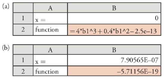
Next, we set up the spreadsheet shown in Figure \(\PageIndex{1}\)a, placing the formula for the cubic equation in cell B2, and entering our initial guess for x in cell B1. Because Pb(IO3)2 is not very soluble, we expect that x is small and set our initial guess to 0. Finally, we access the Solver function by selecting Solver... from the Tools menu, which opens the Solver Parameters window.
To define the problem, place the cursor in the box for Set Target Cell and then click on cell B2. Select the Value of: radio button and enter 0 in the box. Place the cursor in the box for By Changing Cells: and click on cell B1. Together, these actions instruct the Solver function to change the value of x, which is in cell B1, until the cubic equation in cell B2 equals zero. Before we actually solve the function, we need to consider whether there are any limitations for an acceptable result. For example, we know that x cannot be smaller than 0 because a negative concentration is not possible. We also want to ensure that the solution’s precision is acceptable. Click on the button labeled Options... to open the Solver Options window. Checking the option for Assume Non-Negative forces the Solver to maintain a positive value for the contents of cell B1, meeting one of our criteria. Setting the precision requires a bit more thought. The Solver function uses the precision to decide when to stop its search, doing so when
\[|\text { expected value }-\text { calculated value } | \times 100=\text { precision }(\%) \nonumber\]
where expected value is the target cell’s desired value (0 in this case), calculated value is the function’s current value (cell B1 in this case), and precision is the value we enter in the box for Precision. Because our initial guess of x = 0 gives a calculated result of \(2.5 \times 10^{-13}\), accepting the Solver’s default precision of \(1 \times 10^{-6}\) will stop the search after one cycle. To be safe, let’s set the precision to \(1 \times 10^{-18}\). Click OK and then Solve. When the Solver function finds a solution, the results appear in your spreadsheet (see Figure \(\PageIndex{1}\)b). Click OK to keep the result, or Cancel to return to the original values. Note that the answer here agrees with our earlier result of \(7.91 \times 10^{-7}\) M for the solubility of Pb(IO3)2.
Be sure to evaluate the reasonableness of Solver’s answer. If necessary, repeat the process using a smaller value for the precision.
Example 2: pH of 1.0 M HF
In developing our earlier solution to this problem we began by identifying four unknowns and writing out the following four equations.
\[K_{\mathrm{a}}=\frac{\left[\mathrm{H}_{3} \mathrm{O}^{+}\right]\left[\mathrm{F}^{-}\right]}{[\mathrm{HF}]}=6.8 \times 10^{-4} \nonumber\]
\[K_{w}=\left[\mathrm{H}_{3} \mathrm{O}^{+}\right]\left[\mathrm{OH}^{-}\right]=1.00 \times 10^{-14} \nonumber\]
\[C_{\mathrm{HF}}=[\mathrm{HF}]+\left[\mathrm{F}^{-}\right] \nonumber\]
\[\left[\mathrm{H}_{3} \mathrm{O}^{+}\right]=\left[\mathrm{OH}^{-}\right]+\left[\mathrm{F}^{-}\right] \nonumber\]
Next, we made two assumptions that allowed us to simplify the problem to an equation that is easy to solve.
\[\left[\mathrm{H}_{3} \mathrm{O}^{+}\right]=\sqrt{K_{\mathrm{a}} C_{\mathrm{HF}}}=\sqrt{\left(6.8 \times 10^{-4}\right)(1.0)}=2.6 \times 10^{-2} \nonumber\]
Although we did not note this at the time, without making assumptions the solution to our problem is a cubic equation
\[\left[\mathrm{H}_{3} \mathrm{O}^{+}\right]^{3}+K_{\mathrm{a}}\left[\mathrm{H}_{3} \mathrm{O}^{+}\right]^{2}- \left(K_{a} C_{\mathrm{HF}}+K_{\mathrm{w}}\right)\left[\mathrm{H}_{3} \mathrm{O}^{+}\right]-K_{\mathrm{a}} K_{\mathrm{w}}=0 \label{6.1}\]
that we can solve using Excel’s Solver function. Of course, this assumes that we successfully complete the derivation!
Another option is to use Excel to solve the four equations simultaneously by iterating in on values for [HF], [F–], [H3O+], and [OH–]. Figure \(\PageIndex{2}\)a shows a spreadsheet for this purpose. The cells in the first row contain initial guesses for the equilibrium pH. Using the ladder diagram in Figure 6.8.1, pH values between 1 and 3 seems reasonable. You can add additional columns if you wish to include more pH values. The formulas in rows 2–5 use the definition of pH to calculate [H3O+], Kw to calculate [OH–], the charge balance equation to calculate [F–], and Ka to calculate [HF]. To evaluate the initial guesses, we use the mass balance expression for HF, rewriting it as
\[[\mathrm{HF}]+\left[\mathrm{F}^{-}\right]-C_{\mathrm{HF}}=[\mathrm{HF}]+[\mathrm{F}]-1.0=0 \nonumber\]
and entering it in the last row; the values in these cells gives the calculation’s error for each pH.

Figure \(\PageIndex{2}\)b shows the actual values for the spreadsheet in Figure \(\PageIndex{2}\)a. The negative value in cells B6 and C6 means that the combined concentrations of HF and F– are too small, and the positive value in cell D6 means that their combined concentrations are too large. The actual pH, therefore, is between 1.00 and 2.00. Using these pH values as new limits for the spreadsheet’s first row, we continue to narrow the range for the actual pH. Figure \(\PageIndex{2}\)c shows a final set of guesses, with the actual pH falling between 1.59 and 1.58. Because the error for 1.59 is smaller than that for 1.58, we accept a pH of 1.59 as the answer. Note that this is an agreement with our earlier result.
You also can solve this set of simultaneous equations using Excel’s Solver function. To do so, create the spreadsheet in Figure \(\PageIndex{2}\)a, but omit all columns other than A and B. Select Solver... from the Tools menu and define the problem by using B6 for Set Target Cell, setting its desired value to 0, and selecting B1 for By Changing Cells:. You may need to play with the Solver’s options to find a suitable solution to the problem, and it is wise to try several different initial guesses. The Solver function works well for relatively simple problems, such as finding the pH of 1.0 M HF. As problems become more complex and include more unknowns, the Solver function becomes a less reliable tool for solving equilibrium problems.
Using Excel, calculate the solubility of AgI in 0.10 M NH3 without making any assumptions. See our earlier treatment of this problem for the relevant equilibrium reactions and constants.
- Answer
-
For a list of the relevant equilibrium reactions and equilibrium constants, see our earlier treatment of this problem. To solve this problem using Excel, let’s set up the following spreadsheet
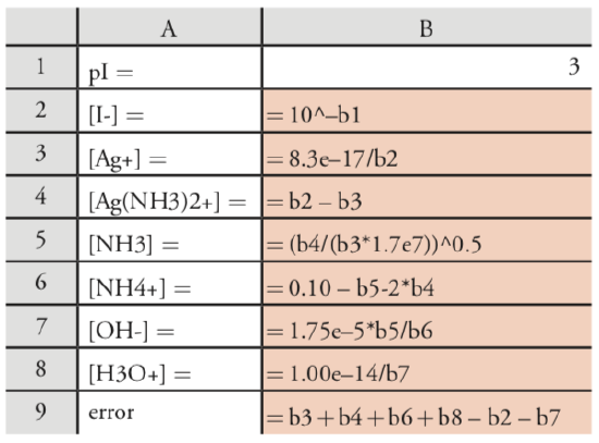
copying the contents of cells B1‐B9 into several additional columns. The initial guess for pI in cell B1 gives the concentration of I– in cell B2. Cells B3–B8 calculate the remaining concentrations, using the Ksp to obtain [Ag+], using the mass balance on iodide and silver to obtain [\(\text{Ag(NH}_3)_2^+\)], using b2 to calculate [NH3], using the mass balance on ammonia to find [\(\text{NH}_4^+\)], using Kb to calculate [OH–], and using Kw to calculate [H3O+]. The system’s charge balance equation provides a means for determining the calculation’s error.
\[\left[\mathrm{Ag}^{+}\right]+\left[\mathrm{Ag}\left(\mathrm{NH}_{3}\right)_{2}^{+}\right]+\left[\mathrm{NH}_{4}^{+}\right]+\left[\mathrm{H}_{3} \mathrm{O}^{+}\right]-\left[\mathrm{I}^{-}\right]+\left[\mathrm{OH}^{-}\right]=0 \nonumber\]
The largest possible value for pI, which corresponds to the smallest concentration of I– and the lowest possible solubility, occurs for a simple, saturated solution of AgI. When [Ag+] = [I–], the concentration of iodide is
\[\left[\mathrm{I}^{-}\right]=\sqrt{K_{\mathrm{sp}}}=\sqrt{8.3 \times 10^{-17}}=9.1 \times 10^{-9} \nonumber\]
which corresponds to a pI of 8.04. Entering initial guesses for pI of 4, 5, 6, 7, and 8 shows that the error changes sign between a pI of 5 and 6. Continuing in this way to narrow down the range for pI, we find that the error function is closest to zero at a pI of 5.42. The concentration of I– at equilibrium, and the molar solubility of AgI, is \(3.8 \times 10^{-6}\) mol/L, which agrees with our earlier solution to this problem.
R
R has a simple command—uniroot—for finding the chemically significant root of a polynomial equation. In addition, it is easy to write a function to solve a set of simultaneous equations by iterating in on a solution. Let’s work through two examples.
Example 1: Solubility of Pb(IO3)2 in 0.10 M Pb(NO3)2
In our earlier treatment of this problem we arrived at the following cubic equation
\[4 x^{3}+0.40 x^{2}=2.5 \times 10^{-13} \nonumber\]
where x is the equilibrium concentration of Pb2+. Although there are several approaches for solving cubic equations with paper and pencil, none are computationally easy. One approach to solving the problem is to iterate in on the answer by finding two values of x, one that leads to a result larger than \(2.5 \times 10^{-13}\) and one that gives a result smaller than \(2.5 \times 10^{-13}\). Having established boundaries for the value of x, we then shift the upper limit and the lower limit until the precision of our answer is satisfactory. Without going into details, this is how the uniroot command works.
The general form of the uniroot command is
uniroot(function, lower, upper, tol)
where function is an object that contains the equation whose root we seek, lower and upper are boundaries for the root, and tol is the desired precision for the root. To create an object that contains the equation, we rewrite it so that its right‐side equals zero.
\[4 x^{3}+0.40 x^{2}-2.5 \times 10^{-13} = 0 \nonumber\]
Next, we enter the following code, which defines our cubic equation as a function with the name eqn.
> eqn = function(x) {4*x^3 + 0.4*x^2 – 2.5e–13}
Because our equation is a function, the uniroot command can send a value of x to eqn and receive back the equation’s corresponding value.
For example, entering
> eqn(2)
passes the value x = 2 to the function and returns an answer of 33.6.
Finally, we use the uniroot command to find the root.
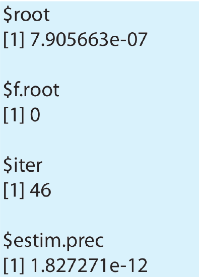
> uniroot(eqn, lower = 0, upper = 0.1, tol = 1e–18)
Because Pb(IO3)2 is not very soluble, we expect that x is small and set the lower limit to 0. The choice for the upper limit is less critical. To ensure that the solution has sufficient precision, we set the tolerance to a value that is smaller than the expected root. Figure \(\PageIndex{3}\) shows the resulting output. The value $root is the equation’s root, which is in good agreement with our earlier result of \(7.91 \times 10^{-7}\) for the molar solubility of Pb(IO3)2. The other results are the equation’s value for the root, the number of iterations needed to find the root, and the root’s estimated precision.
Example 2: pH of 1.0 M HF
In developing our earlier solution to this problem we began by identifying four unknowns and writing out the following four equations.
\[K_{\mathrm{a}}=\frac{\left[\mathrm{H}_{3} \mathrm{O}^{+}\right]\left[\mathrm{F}^{-}\right]}{[\mathrm{HF}]}=6.8 \times 10^{-4} \nonumber\]
\[K_{w}=\left[\mathrm{H}_{3} \mathrm{O}^{+}\right]\left[\mathrm{OH}^{-}\right]=1.00 \times 10^{-14} \nonumber\]
\[C_{\mathrm{HF}}=[\mathrm{HF}]+\left[\mathrm{F}^{-}\right] \nonumber\]
\[\left[\mathrm{H}_{3} \mathrm{O}^{+}\right]=\left[\mathrm{OH}^{-}\right]+\left[\mathrm{F}^{-}\right] \nonumber\]
Next, we made two assumptions that allowed us to simplify the problem to an equation that is easy to solve.
\[\left[\mathrm{H}_{3} \mathrm{O}^{+}\right]=\sqrt{K_{\mathrm{a}} C_{\mathrm{HF}}}=\sqrt{\left(6.8 \times 10^{-4}\right)(1.0)}=2.6 \times 10^{-2} \nonumber\]
Although we did not note this at the time, without making assumptions the solution to our problem is a cubic equation
\[\left[\mathrm{H}_{3} \mathrm{O}^{+}\right]^{3}+K_{\mathrm{a}}\left[\mathrm{H}_{3} \mathrm{O}^{+}\right]^{2}- \left(K_{a} C_{\mathrm{HF}}+K_{\mathrm{w}}\right)\left[\mathrm{H}_{3} \mathrm{O}^{+}\right]-K_{\mathrm{a}} K_{\mathrm{w}}=0 \nonumber\]
that we can solve using the uniroot command. Of course, this assumes that we successfully complete the derivation!
Another option is to write a function to solve the four equations simultaneously. Here is the code for this function, which we will call eval.
> eval = function(pH){
+ h3o = 10^–pH
+ oh = 1e–14/h3o
+ hf = (h3o * f )/6.8e–4
+ error= hf + f – 1
+ output= data.frame(pH, error)
+ print(output)
+}
The open curly braces, {, tells R that we intend to enter our function over several lines. When we press enter at the end of a line, R changes its prompt from > to +, indicating that we are continuing to enter the same command. The closed curly brace, }, on the last line indicates that we have completed the function. The command data.frame combines two or more objects into a table, which we then print out so that we can view the results of the calculations. You can adapt this function to other problems by changing the variable you pass to the function and the equations you include within the function.
Let’s examine more closely how this function works. The function accepts a guess for the pH and uses the definition of pH to calculate [H3O+], Kw to calculate [OH–], the charge balance equation to calculate [F–], and Ka to calculate [HF]. The function then evaluates the solution using the mass balance expression for HF, rewriting it as
\[[\mathrm{HF}]+\left[\mathrm{F}^{-}\right]-C_{\mathrm{HF}}=[\mathrm{HF}]+\left[\mathrm{F}^{-}\right]-1.0=0 \nonumber\]
The function then gathers together the initial guess for the pH and the error and prints them as a table.
The beauty of this function is that the object we pass to it, pH, can contain many values, which makes it easy to search for a solution. Because HF is an acid, we know that the solution is acidic. This sets an upper limit of 7 for the pH. We also know that the pH of 1.0 M HF is no smaller than 0 as this is the pH if HF was a strong acid. For our first pass, let’s enter the following code
> pH= c(7, 6, 5, 4, 3, 2, 1)
> eval(pH)
which varies the pH within these limits. The result, which is shown in Figure \(\PageIndex{4}\)a, indicates that the pH is less than 2 and greater than 1 because it is in this interval that the error changes sign.
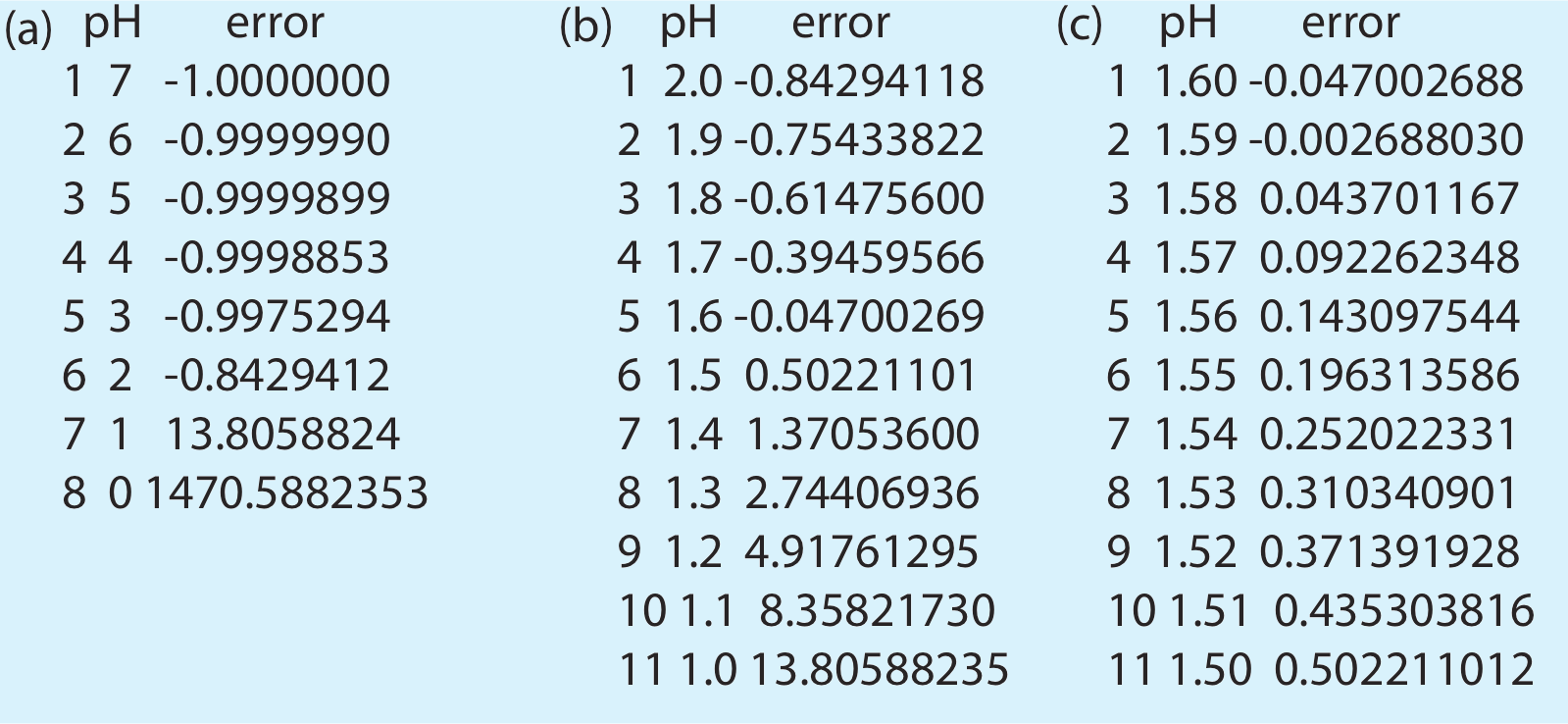
For our second pass, let’s explore pH values between 2.0 and 1.0 to further narrow down the problem’s solution.
> pH = c(2.0, 1.9, 1.8, 1.7, 1.6, 1.5, 1.4, 1.3, 1.2, 1.1, 1.0)
> eval(pH)
The result in Figure \(\PageIndex{4}\)b show that the pH must be less than 1.6 and greater than 1.5. A third pass between these limits gives the result shown in Figure \(\PageIndex{4}\)c, which is consistent with our earlier result of a pH 1.59.
Using R, calculate the solubility of AgI in 0.10 M NH3 without making any assumptions. See our earlier treatment of this problem for the relevant equilibrium reactions and constants.
- Answer
-
To solve this problem, let’s use the following function
> eval = function(pI){
+ I = 10^–pI
+ Ag = 8.3e–17/I
+ AgNH3 = Ag – I
+ NH3 = (AgNH3/(1.7e7*Ag))^0.5
+ NH4 = 0.10‐NH3 – 2 * AgNH3
+ OH = 1.75e–5 * NH3/NH4
+ H3O = 1e–14/OH
+ error = Ag + AgNH3 + NH4 + H3O – OH – I
+ output = data.frame(pI, error)
+ print(output)
+}
The function accepts an initial guess for pI and calculates the concentrations of each species in solution using the definition of pI to calculate [I–], using the Ksp to obtain [Ag+], using the mass balance on iodide and silver to obtain [\(\text{Ag(NH}_3)_2^+\)], using \(\beta_2\) to calculate [NH3], using the mass balance on ammonia to find [\(\text{NH}_4^+\)], using Kb to calculate [OH–], and using Kw to calculate [H3O+]. The system’s charge balance equation provides a means for determining the calculation’s error.
\[\left[\mathrm{Ag}^{+}\right]+\left[\mathrm{Ag}\left(\mathrm{NH}_{3}\right)_{2}^{+}\right]+\left[\mathrm{NH}_{4}^{+}\right]+\left[\mathrm{H}_{3} \mathrm{O}^{+}\right]-\left[\mathrm{I}^{-}\right]+\left[\mathrm{OH}^{-}\right]=0 \nonumber\]
The largest possible value for pI—corresponding to the smallest concentration of I– and the lowest possible solubility—occurs for a simple, saturated solution of AgI. When [Ag+] = [I–], the concentration of iodide is
\[\left[\mathrm{I}^{-}\right]=\sqrt{K_{\mathrm{sp}}}=\sqrt{8.3 \times 10^{-17}}=9.1 \times 10^{-9} \nonumber\]
corresponding to a pI of 8.04. The following session shows the function in action.
> pI=c(4, 5, 6, 7, 8)
> eval(pI)
pI error
1 4 ‐2.56235615
2 5 ‐0.16620930
3 6 0.07337101
4 7 0.09734824
5 8 0.09989073
> pI =c(5.1, 5.2, 5.3, 5.4, 5.5, 5.6, 5.7, 5.8, 5.9, 6.0)> eval(pI)
pI error
1 5.1 ‐0.111446582 5.2 ‐0.06794105
3 5.3 ‐0.03336475
4 5.4 ‐0.00568116
5 5.5 0.01571549
6 5.6 0.03308929
7 5.7 0.04685937
8 5.8 0.05779214
9 5.9 0.06647475
10 6.0 0.07337101> pI =c(5.40, 5.41, 5.42, 5.43, 5.44, 5.45, 5.46, 5.47, 5.48, 5.49, 5.50)
> eval(pI)
pI error
1 5.40 ‐0.0056811605
2 5.41 ‐0.0030715484
3 5.42 0.0002310369
4 5.43 ‐0.0005134898
5 5.44 0.0028281878
6 5.45 0.0052370980
7 5.46 0.0074758181
8 5.47 0.0096260370
9 5.48 0.0117105498
10 5.49 0.0137387291
11 5.50 0.0157154889
The error function is closest to zero at a pI of 5.42. The concentration of I– at equilibrium, and the molar solubility of AgI, is \(3.8 \times 10^{-6}\) mol/L, which agrees with our earlier solution to this problem.