
19: More on Hydrogen Wavefunction, Electronic Spectroscopy and Effective Charge
- Page ID
- 198584

\( \newcommand{\vecs}[1]{\overset { \scriptstyle \rightharpoonup} {\mathbf{#1}} } \)
\( \newcommand{\vecd}[1]{\overset{-\!-\!\rightharpoonup}{\vphantom{a}\smash {#1}}} \)
\( \newcommand{\dsum}{\displaystyle\sum\limits} \)
\( \newcommand{\dint}{\displaystyle\int\limits} \)
\( \newcommand{\dlim}{\displaystyle\lim\limits} \)
\( \newcommand{\id}{\mathrm{id}}\) \( \newcommand{\Span}{\mathrm{span}}\)
( \newcommand{\kernel}{\mathrm{null}\,}\) \( \newcommand{\range}{\mathrm{range}\,}\)
\( \newcommand{\RealPart}{\mathrm{Re}}\) \( \newcommand{\ImaginaryPart}{\mathrm{Im}}\)
\( \newcommand{\Argument}{\mathrm{Arg}}\) \( \newcommand{\norm}[1]{\| #1 \|}\)
\( \newcommand{\inner}[2]{\langle #1, #2 \rangle}\)
\( \newcommand{\Span}{\mathrm{span}}\)
\( \newcommand{\id}{\mathrm{id}}\)
\( \newcommand{\Span}{\mathrm{span}}\)
\( \newcommand{\kernel}{\mathrm{null}\,}\)
\( \newcommand{\range}{\mathrm{range}\,}\)
\( \newcommand{\RealPart}{\mathrm{Re}}\)
\( \newcommand{\ImaginaryPart}{\mathrm{Im}}\)
\( \newcommand{\Argument}{\mathrm{Arg}}\)
\( \newcommand{\norm}[1]{\| #1 \|}\)
\( \newcommand{\inner}[2]{\langle #1, #2 \rangle}\)
\( \newcommand{\Span}{\mathrm{span}}\) \( \newcommand{\AA}{\unicode[.8,0]{x212B}}\)
\( \newcommand{\vectorA}[1]{\vec{#1}} % arrow\)
\( \newcommand{\vectorAt}[1]{\vec{\text{#1}}} % arrow\)
\( \newcommand{\vectorB}[1]{\overset { \scriptstyle \rightharpoonup} {\mathbf{#1}} } \)
\( \newcommand{\vectorC}[1]{\textbf{#1}} \)
\( \newcommand{\vectorD}[1]{\overrightarrow{#1}} \)
\( \newcommand{\vectorDt}[1]{\overrightarrow{\text{#1}}} \)
\( \newcommand{\vectE}[1]{\overset{-\!-\!\rightharpoonup}{\vphantom{a}\smash{\mathbf {#1}}}} \)
\( \newcommand{\vecs}[1]{\overset { \scriptstyle \rightharpoonup} {\mathbf{#1}} } \)
\(\newcommand{\longvect}{\overrightarrow}\)
\( \newcommand{\vecd}[1]{\overset{-\!-\!\rightharpoonup}{\vphantom{a}\smash {#1}}} \)
\(\newcommand{\avec}{\mathbf a}\) \(\newcommand{\bvec}{\mathbf b}\) \(\newcommand{\cvec}{\mathbf c}\) \(\newcommand{\dvec}{\mathbf d}\) \(\newcommand{\dtil}{\widetilde{\mathbf d}}\) \(\newcommand{\evec}{\mathbf e}\) \(\newcommand{\fvec}{\mathbf f}\) \(\newcommand{\nvec}{\mathbf n}\) \(\newcommand{\pvec}{\mathbf p}\) \(\newcommand{\qvec}{\mathbf q}\) \(\newcommand{\svec}{\mathbf s}\) \(\newcommand{\tvec}{\mathbf t}\) \(\newcommand{\uvec}{\mathbf u}\) \(\newcommand{\vvec}{\mathbf v}\) \(\newcommand{\wvec}{\mathbf w}\) \(\newcommand{\xvec}{\mathbf x}\) \(\newcommand{\yvec}{\mathbf y}\) \(\newcommand{\zvec}{\mathbf z}\) \(\newcommand{\rvec}{\mathbf r}\) \(\newcommand{\mvec}{\mathbf m}\) \(\newcommand{\zerovec}{\mathbf 0}\) \(\newcommand{\onevec}{\mathbf 1}\) \(\newcommand{\real}{\mathbb R}\) \(\newcommand{\twovec}[2]{\left[\begin{array}{r}#1 \\ #2 \end{array}\right]}\) \(\newcommand{\ctwovec}[2]{\left[\begin{array}{c}#1 \\ #2 \end{array}\right]}\) \(\newcommand{\threevec}[3]{\left[\begin{array}{r}#1 \\ #2 \\ #3 \end{array}\right]}\) \(\newcommand{\cthreevec}[3]{\left[\begin{array}{c}#1 \\ #2 \\ #3 \end{array}\right]}\) \(\newcommand{\fourvec}[4]{\left[\begin{array}{r}#1 \\ #2 \\ #3 \\ #4 \end{array}\right]}\) \(\newcommand{\cfourvec}[4]{\left[\begin{array}{c}#1 \\ #2 \\ #3 \\ #4 \end{array}\right]}\) \(\newcommand{\fivevec}[5]{\left[\begin{array}{r}#1 \\ #2 \\ #3 \\ #4 \\ #5 \\ \end{array}\right]}\) \(\newcommand{\cfivevec}[5]{\left[\begin{array}{c}#1 \\ #2 \\ #3 \\ #4 \\ #5 \\ \end{array}\right]}\) \(\newcommand{\mattwo}[4]{\left[\begin{array}{rr}#1 \amp #2 \\ #3 \amp #4 \\ \end{array}\right]}\) \(\newcommand{\laspan}[1]{\text{Span}\{#1\}}\) \(\newcommand{\bcal}{\cal B}\) \(\newcommand{\ccal}{\cal C}\) \(\newcommand{\scal}{\cal S}\) \(\newcommand{\wcal}{\cal W}\) \(\newcommand{\ecal}{\cal E}\) \(\newcommand{\coords}[2]{\left\{#1\right\}_{#2}}\) \(\newcommand{\gray}[1]{\color{gray}{#1}}\) \(\newcommand{\lgray}[1]{\color{lightgray}{#1}}\) \(\newcommand{\rank}{\operatorname{rank}}\) \(\newcommand{\row}{\text{Row}}\) \(\newcommand{\col}{\text{Col}}\) \(\renewcommand{\row}{\text{Row}}\) \(\newcommand{\nul}{\text{Nul}}\) \(\newcommand{\var}{\text{Var}}\) \(\newcommand{\corr}{\text{corr}}\) \(\newcommand{\len}[1]{\left|#1\right|}\) \(\newcommand{\bbar}{\overline{\bvec}}\) \(\newcommand{\bhat}{\widehat{\bvec}}\) \(\newcommand{\bperp}{\bvec^\perp}\) \(\newcommand{\xhat}{\widehat{\xvec}}\) \(\newcommand{\vhat}{\widehat{\vvec}}\) \(\newcommand{\uhat}{\widehat{\uvec}}\) \(\newcommand{\what}{\widehat{\wvec}}\) \(\newcommand{\Sighat}{\widehat{\Sigma}}\) \(\newcommand{\lt}{<}\) \(\newcommand{\gt}{>}\) \(\newcommand{\amp}{&}\) \(\definecolor{fillinmathshade}{gray}{0.9}\)Recap of Lecture 18
Last Lecture addressed the angular moment of an electron revolving around the nucleus. This is described by the \(l\) quantum number and an electron in any non-spherical orbital (i.e., an s orbital) will have an angular moment (you should know formula). The \(m_{\ell}\) quantum number designates the orientation of that angular moment wrt the z-axis (and there is a formula for that too) and the degeneracy can be partial broken by magnetic fields. We discussed that we cannot always do a one-to-one correspondence between quantum numbers to orbitals. We discussed basic spectroscopy of H-like system and specifically selection rules (for n,l, and ml). We introduced the He system, discussed we cannot solve it and need to do approximations. We discussed the first approximation, which is the worst possible one.
The \(m_{\ell}\) Quantum Number and Magnetic Fields
The magnetic quantum number, designated by the letter \(m_{\ell}\), is the third quantum numbers which describe the unique quantum state of an electron. The magnetic quantum number distinguishes the orbitals available within a subshell, and is used to calculate the azimuthal component of the orientation of the orbital in space. As with our discussion of rigid rotors, the quantum number \(m_{\ell}\) refers to the projection of the angular momentum in this arbitrarily chosen direction, conventionally called the \(z\) direction or quantization axis. \(L_z\), the magnitude of the angular momentum in the z direction, is given by the formula
\[ L_z = m_{\ell} \hbar \label{eq1}\]
The quantum number \(m_{\ell}\) refers, loosely, to the direction of the angular momentum vector. The magnetic quantum number \(m_{\ell}\) only affects the electron's energy if it is in a magnetic field because in the absence of one, all spherical harmonics corresponding to the different arbitrary values of \(m_{\ell}\) are equivalent.
Zeeman Effect
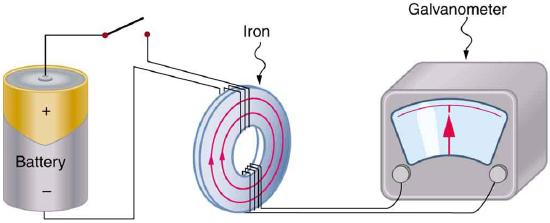
Magnetism results from the circular motion of charged particles. This property is demonstrated on a macroscopic scale by making an electromagnet from a coil of wire and a battery. Electrons moving through the coil produce a magnetic field, which can be thought of as originating from a magnetic dipole or a bar magnet.
Electrons in atoms also are moving charges with angular momentum so they too produce a magnetic dipole, which is why some materials are magnetic. A magnetic dipole interacts with an applied magnetic field, and the energy of this interaction is given by the scalar product of the magnetic dipole moment (magnetic moment (\(\vec{\mu _m}\) ) and the magnetic field, \(\vec{B}\).
\[E_B = - \vec{\mu} _m \cdot \vec{B} \label {8.4.1}\]
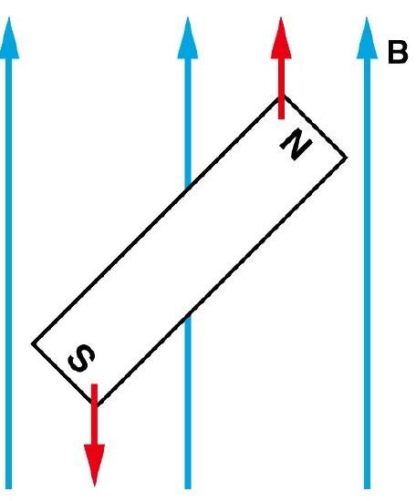
Magnets are acted on by forces and torques when placed within an external applied magnetic field (Figure \(\PageIndex{2}\)). In a uniform external field, a magnet experiences no net force, but a net torque. The torque tries to align the magnetic moment (\(\vec{\mu} _m\) of the magnet with the external field \(\vec{B}\). The magnetic moment of a magnet points from its south pole to its north pole.
The magnetic quantum number determines the energy shift of an atomic orbital due to an external magnetic field (this is called the Zeeman effect) — hence the name magnetic quantum number. However, the actual magnetic dipole moment of an electron in an atomic orbital arrives not only from the electron angular momentum, but also from the electron spin, expressed in the spin quantum number, which is the fourth quantum number. \(m_s\) and discussed in the next chapter.
Example \(\PageIndex{1}\)
Electrons with non-zero angular momenta exhibit magnetic moments, which depend on the specific wavefunctions the electrons occupy (and specifically the \(\ell\) quantum number). In the absence of an external magnetic field, different orientations of this magnetic field (i.e., electrons in wavefunctions with different \(m_{\ell}) values) will have the same energy. In the presence of an external field, the degeneracy of these different wavefunctions break. Assume the external magnetic field is oriented in the z-direction, predict the splitting patterns for an electron in the following orbitals:
- 1s orbital
- 2p orbitals (consider each orbital)
- 2s orbital
- 3d orbitals (consider each orbital)
- How do you think the splitting would be for a helium atom?
Which \(m_{\ell}\) number corresponds to which \(p\)-orbital?
The answer is complicated; while \(m_{\ell}=0\) corresponds to the \(p_z\), the orbitals for \(m_{\ell}=+1\) and \(m_{\ell}=−1\) lie in the xy-plane (see Spherical Harmonics), but not on the axes. The reason for this outcome is that the wavefunctions are usually formulated in spherical coordinates to make the math easier, but graphs in the Cartesian coordinates make more intuitive sense for humans. The \(p_x\) and \(p_y\) orbitals are constructed via a linear combination approach from radial and angular wavefunctions and converted into \(xy\) (this was discussed previously). Thus, it is not possible to directly correlate the values of \(m_{\ell}=±1\) with specific orbitals.
Note: We sometimes lie to students
The notion that we can directly correlate the values of \(m_{\ell}=±1\) with specific orbitals is sometimes presented in introductory courses (not the Libretexts) to make a complex mathematical model just a little bit simpler and more intuitive, but it is incorrect.
The three wavefunctions for \(n=2\) and \(\ell=1\) are as follows (the spherical harmonics).
\[ \begin{align*} |Ψ_{2,1,0} \rangle &=r \cos θR(r) \\[4pt] |Ψ_{2,1,+1} \rangle &=−\dfrac{r}{2} \sinθ e^{iϕ} R(r) \\[4pt] |Ψ_{2,1,-1} \rangle &=+\dfrac{r}{2} \sinθ e^{-iϕ} R(r) \end{align*}\]
The notation is \(|Ψ_{n,l,m_{\ell}} \rangle\) with \(R(r)\) is the radial component of this wavefuction, \(θ\) is the angle with respect to the z-axis and \(ϕ\) is the angle with respect to the \(xz\)-plane.
\[R(r)=\sqrt{\dfrac{Z^5}{32\pi a_0^5}}\mathrm{e}^{-Zr/2a_0}\]
in which \(Z\) is the atomic number (or probably better nuclear charge) and \(a_0\) is the Bohr radius.
In switching from spherical to Cartesian coordinates, we make the substitution \(z=r \cos θ\), so:
\[|Ψ_{2,1,0} \rangle =z R(r)\]
This is \(Ψ_{2p_z}\) since the value of \(Ψ\) is dependent on \(z\): when \(z=0\); \(Ψ=0\), which is expected since \(z=0\) describes the \(xy\)-plane.
The other two wavefunctions are degenerate in the \(xy\)-plane. An equivalent statement is that these two orbitals do not lie on the x- and y-axes, but rather bisect them. Thus it is typical to take linear combinations of them to make the equations real and easier to conceptualize. We can do this because of the linearity of the Schrödinger equation.
If any set of wavefunctions is a solution to the Schrödinger equation, then any set of linear combinations of these wavefunctions must also be a solution.
In the equations below, we're going to make use of some trigonometry, notably Euler's formula:
\[\mathrm{e}^{\mathrm{i}\phi}=\cos{\phi}+\mathrm{i}\sin{\phi}\]
\[\sin{\phi} = \frac{\mathrm{e}^{\mathrm{i}\phi}-\mathrm{e}^{-\mathrm{i}\phi}}{2\mathrm{i}}\]
\[\cos{\phi} = \frac{\mathrm{e}^{\mathrm{i}\phi}+\mathrm{e}^{-\mathrm{i}\phi}}{2}\]
We're also going to use \(x=\sin θ\cos ϕ\) and \(y=\sin θ \sinϕ \).
\begin{align} \psi_{2p_x}=\frac{1}{\sqrt{2}}\left(\psi_{2,1,+1}-\psi_{2,1,-1}\right)=\frac{1}{2}\left(\mathrm{e}^{\mathrm{i}\phi}+\mathrm{e}^{-\mathrm{i}\phi} \right)r\sin{\theta}f(r)=r\sin{\theta}\cos{\phi}f(r)=xf(r) \\ \psi_{2p_y}=\frac{\mathrm{i}}{\sqrt{2}}\left(\psi_{2,1,+1}+\psi_{2,1,-1}\right)=\frac{1}{2\mathrm{i}}\left(\mathrm{e}^{\mathrm{i}\phi}-\mathrm{e}^{-\mathrm{i}\phi} \right)r\sin{\theta}f(r)=r\sin{\theta}\sin{\phi}f(r)=yf(r)\\ \end{align}
So, while \(m_{\ell}=0\) corresponds to \(|p_z \rangle\), \(m_{\ell}=+1\) and \(m_{\ell}=−1\) cannot be directly assigned to \(|p_x \rangle\) and \(|p_y \rangle\).
Rather \(m_{\ell}=\pm 1\) corresponds to {\(p_x \rangle\), \(p_y \rangle\)}. An alternative discription is that \(m_{\ell}=+1\) might correspond to \((|p_x \rangle\ + |p_y \rangle )\) and \(m_{\ell}=−1\) might correspond to \((|p_x \rangle\ - |p_y \rangle)\).
The Math is the same for Solving any Hydrogen-like (One electron) ion
The Hamiltonian for a one electron atom is given by is given by
\[\hat{H}_{electron} = -\dfrac {\hbar^2}{2\mu} \bigtriangledown^2 - \dfrac {Ze^2}{4\pi \epsilon_0 r}\label{7}\]
This only differs by the \(Z^2\) component from the hydrogen atom.
Solving \(\hat{H}\psi_n = E_n \psi_n\) gives \(E=-RZ^2/n^2\).
For example with He+, the 2s orbital
\(E_{He_{2s}}\) has \(z=2, n=2\), thus \(E_{He_{2s}} = -R\)
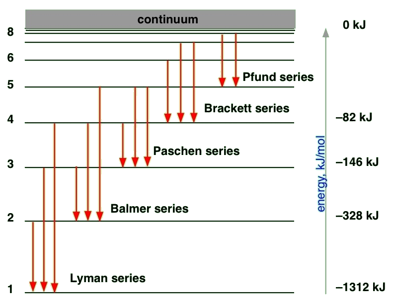
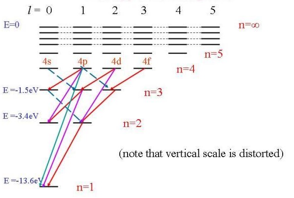
Spectroscopy of Hydrogen atoms
The solution of the Schrödinger equation for the hydrogen atom predicts that energy levels with \(n > 1\) can have several orbitals with the same energy. In fact, as the energy and n increase, the degeneracy of the orbital energy level increases as well. The number of orbitals with a particular energy and value for \(n\) is given by \(n_2\). Thus, each orbital energy level is predicted to be \(n_2\)-degenerate. This high degree of orbital degeneracy is predicted only for one-electron systems. For multi-electron atoms, the electron-electron repulsion removes the \(l\) degeneracy so only orbitals with the same \(m_{\ell}\) quantum numbers are degenerate.
To understand the hydrogen atom spectrum, we also need to determine which transitions are allowed and which transitions are forbidden. This issue is addressed next by using selection rules that are obtained from the transition moment integral. Previously, we determined selection rules for the particle in a box, the harmonic oscillator, and the rigid rotor. Now we will apply those same principles to the hydrogen atom case by starting with the transition moment integral.
Transition requires a transfer from one state with its quantum numbers \((n_i, l_i, m_i)\) to another state \((n_f, l_f, m_f)\). The transition moment integral for a transition between an initial (\(i\)) state and a final (\(f\)) state of a hydrogen atom is given by
\[ \left \langle \mu _T \right \rangle = \int \psi ^* _{n_f, l_f, m_{l_f}} (r, \theta , \psi ) \hat {\mu} \psi _{n_i, l_i, m_{l_i}} (r, \theta , \psi ) d \tau \label {8.3.2a}\]
or in bra ket notation
\[ \left \langle \mu _T \right \rangle = \langle \psi ^*_{n_f, l_f, m_{l_f}} | \hat {\mu} | \psi _{n_i, l_i, m_{l_i}} \rangle \label{8.3.2b}\]
where the dipole moment operator is given by
\[ \hat {\mu} = - e \hat {r} \label {8.3.3}\]
The dipole moment operator expressed in spherical coordinates is
\[ \hat {\mu} = -er (\bar {x} \sin \theta \cos \psi + \bar {y} \sin \theta \sin \psi + \bar {z} \cos \theta \label {8.3.4}\]
The right hand side of Equation \ref{8.3.4} shows that there are three components of \(\left \langle \mu _T \right \rangle\) to evaluate in \ref{8.3.2}, where each component consists of three integrals: an \(r\) integral, a \(\theta \) integral, and a \(\psi \) integral.
Evaluation reveals that the \(r\) integral always differs from zero so
\[ \color{red} \Delta n = n_f - n_i = \text {not restricted} \label {8.3.5}\]
There is no restriction on the change in the principal quantum number during a spectroscopic transition; \(\Delta n\) can be anything. For absorption, \(\Delta n > 0 \), for emission \(\Delta n < 0\), and \(\Delta n = 0 \) when the orbital degeneracy is removed by an external field or some other interaction.
The selection rules for \(\Delta l \) and \(\Delta m_{\ell}\) come from the transition moment integrals involving \(\theta \) and \(\varphi\) in Equation (8.3.2). These integrals are the same ones that were evaluated for the rotational selection rules, and the resulting selection rules are
\[ \color{red} \Delta l = \pm 1\]
and
\[ \color{red} \Delta m_{\ell} = 0, \pm 1\]
These rules demand conservation of angular momentum. Since a photon carries an intrinsic angular momentum of 1.
One Electron ion (e.g., Helium+)
The Hamiltonian for a one electron atom is given by is given by
\[\hat{H}_{electron} = -\dfrac {\hbar^2}{2\mu} \bigtriangledown^2 - \dfrac {Ze^2}{4\pi \epsilon_0 r}\]
Solving
\[\hat{H} |\psi_n \rangle = E_n | \psi_n \rangle \]
gives energies of
\(E_n=-R\dfrac{Z^2}{n^2}\).
Which as with the hydrogen atom are degenerate with respect to the \(l\) and \(m_{\ell}\) quantum numbers.
For example with an electron in the 2s orbital of \(He^+\) with \(Z=2, \;n=2\), has an energy:
\[E_{He_{2s}} = -R\]
but the electron in the lowest eigenstate with \(Z=2, \;n=1\) is
\[E_{He_{2s}} = -4R\]
The Eigenvalue Problem for the Helium Atom
Step 1: Define the potential for the problem
\[ V(r_1,r_2) = \underset{\text{nucleaus-electron 1 attraction}}{- \dfrac {Ze^2}{4\pi\epsilon_0 r_1}} - \underset{\text{nucleaus-electron 2 attraction}}{\dfrac {Ze^2}{4\pi\epsilon_0 r_2}} + \underset{\text{electron-electron repulsion}}{\dfrac {e^2}{4\pi \epsilon_0 r_{12}}}\]
where
- \(r_1\) and \(r_2\) are the ditances of electron 1 and electron 2 from the nucleus
- \(r_{12}\) is the distance between the two electrons
- \(Z\) is the proton number (i.e., charge of the nucleas), which for Helium is \(Z=2\)
Step 2: Define the Schrödinger Equation for the problem
With every quantum eigenvalue problem, we define the Hamiltonian as such:
\[\hat {H} = T + V\]
The potential is defined above and the Kinetic energy of each electron is given by
\[T = -\dfrac {\hbar^2}{2m_e} \bigtriangledown^2\]
For a 2 electron atom, the Hamiltonian should consist of the Hamiltonian for two electrons, and an electron repulsion factor, given by
\[\dfrac {e^2}{4\pi\epsilon_0 r_{12}}\]
The \(r_{12}\) term is the distance from electron 1 to electron 2, which is incredibly hard to solve for. The Hamiltonian for the Helium atom is:
\[\hat{H} = -\dfrac{\hbar^2}{2m_e}\bigtriangledown_{el_{1}}^2 -\dfrac{\hbar^2}{2m_e}\bigtriangledown_{el_{2}}^2 - \dfrac {Ze^2}{4\pi\epsilon_0 r_1} - \dfrac {Ze^2}{4\pi\epsilon_0 r_2} + \dfrac {e^2}{4\pi \epsilon_0 r_{12}}\label{8}\]
Since the potential \(V(r_1,r_2)\) has no time-dependence, we can se the time independent Schrödinger Equation to "solve" the QM problem:
\[\hat {H} | \psi (r_1,r_2) \rangle = E | \psi (r_1,r_2) \rangle \]
Step 3: Solve the Schrödinger Equation for the problem
Multi-electron systems are "three (or more) body problems", which we cannot solve analytically. However, we can introduce approximations.
Step 4: Do something with the Eigenstates and associated energies
Let's talk about the solutions and approximations first.
Approximations
The "ignorance is bliss" approximation
Ignore the \(\dfrac {e^2}{4\pi\epsilon_0 r_{12}}\) electron-electron repulsion term. This assume electron 1 is separable from electron 2, so that
\[\psi_{total} = \psi_{el_{1}}\psi_{el_{2}}\]
or in braket notation
\[ | \psi_{total} \rangle = \hat{H} | \psi_{el_1} \rangle | \psi_{el_2} \rangle\]
With some operator algebra, something important arises - the one electron energies are additive:
\[\hat{H} \psi_{total} = (\hat{H}_{el_1} + \hat{H}_{el_2}) \psi_{n\ {el_1}} \psi_{n\ {el_2}} = (E_{n_1} + E_{n_2}) \psi_{n\ {el_1}} \psi_{n\ {el_2}} \]
or in bra-ket notation
\[\hat{H} | \psi_{total} \rangle = \hat{H} | \psi_{el_1} \rangle | \psi_{el_2} \rangle = (E_{n_1} + E_{n_2}) | \psi_{1} \rangle | \psi_{1} \rangle \]
The energy for a ground state Helium atom (both electrons in lowest state) is then
\[E_{He_{1s}} = \underset{\text{energy of single electron in helium}}{E_{n_1}} + \underset{\text{energy of single electron in helium}}{E_{n_2}} = -R\left(\dfrac{Z^2}{1}\right) -R \left(\dfrac{Z^2}{1}\right) = -8R\]
where \(R\) is the Rydberg constant (\(13.6 \; eV\) that also maps the lowest energy of the hydrogen atom and \(Z=2\) for the helium nucleus. Experimentally, we find that the total energy for a ground state Helium atom \(E_{He_{1s}} = -5.8066\,R\). The big difference in results is due to the approximation we used to get to the value of \(-8\;R\). The "ignorance is bliss" approximation overestimates the energy of the helium atom greatly; this is a poor approximation and we need to address electron-electron repulsion properly (or better at least).
The general form of the "Ignorance is Bliss" approximation which almost as wrong as you can be for multi-electron atoms
\[\underbrace{E_{z} = nZ^2E_{z=1}}_{\text{bad approximation}}\]
Electron-electron repulsion results in "Shielding"
One way to take electron-electron repulsion into account is to modify the form of the wavefunction. A logical modification is to change the nuclear charge, \(Z\), in the wavefunctions to an effective nuclear charge, from +2 to a smaller value, \(Z_{eff}=\zeta\). The rationale for making this modification is that one electron partially shields the nuclear charge from the other electron.
Electron-electron shielding leads to a reduced effective nuclear charge. \(Z_{eff}\) is used instead of \(Z\) in radial part of wavefunctions.
A region of negative charge density between one of the electrons and the +2 nucleus makes the potential energy between them more positive (decreases the attraction between them). We can effect this change mathematically by using \(Z_{eff} < 2\) in the wavefunction expression. If the shielding were complete, then \(Z_{eff}\) would equal 1. If there is no shielding, then \(Z_{eff} = 2\). So a way to take into account the electron-electron interaction is by saying it produces a shielding effect. The shielding is not zero, and it isn't complete, so the effective nuclear charge is between one and two.
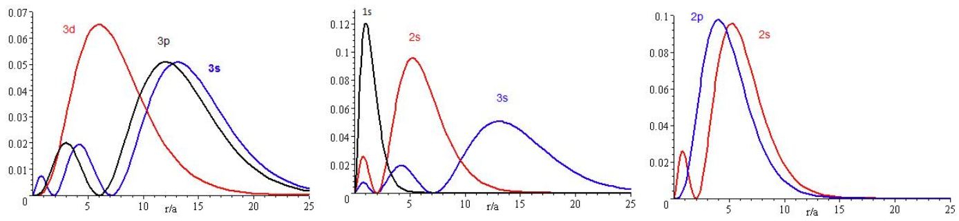
The presence of \(Z_{eff}\) in the radial portions of the wavefunctions also means that the electron probability distributions associated with hydrogenic atomic orbitals in multi-electron systems are different from the exact atomic orbitals for hydrogen. The Figure above compares the radial distribution functions for an electron in a 1s orbital of hydrogen (the ground state), a 2s orbital in hydrogen (an excited configuration of hydrogen) and a 1s orbital in helium that is described by the best variational value of \(Z_{eff}\). Our use of hydrogen-like orbitals in quantum mechanical calculations for multi-electron atoms helps us to interpret our results for multi-electron atoms in terms of the properties of a system we can solve exactly.
Shielding is like attending a Nickelback concert
More electrons create the shielding or screening effect. Shielding or screening means the electrons closer to the nucleus block the outer valence electrons from getting close to the nucleus.
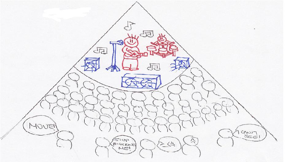
Imagine being in a crowded auditorium in a Nickelback concert. The enthusiastic fans are going to surround the auditorium, trying to get as close to the celebrity on the stage as possible. They are going to prevent people in the back from seeing the celebrity or even the stage. This is shielding. The stage is the nucleus and the celebrity is the protons. The fans are the electrons. Electrons closest to the nucleus will try to be as close to the nucleus as possible. The outer/valence electrons that are farther away from the nucleus will be shielded by the inner electrons. Therefore, the inner electrons prevent the outer electrons from forming a strong attraction to the nucleus. The degree to which the electrons are being screened by inner electrons can be shown by ns<np<nd<nf where n is the energy level. The inner electrons will be attracted to the nucleus much more than the outer electrons. Thus, the attractive forces of the valence electrons to the nucleus are reduced due to the shielding effects. That is why it is easier to remove valence electrons than the inner electrons. It also reduces the nuclear charge of an atom.