
18: Orbital Angular Momentum, Spectroscopy and Multi-Electron Atoms
- Page ID
- 198583

\( \newcommand{\vecs}[1]{\overset { \scriptstyle \rightharpoonup} {\mathbf{#1}} } \)
\( \newcommand{\vecd}[1]{\overset{-\!-\!\rightharpoonup}{\vphantom{a}\smash {#1}}} \)
\( \newcommand{\dsum}{\displaystyle\sum\limits} \)
\( \newcommand{\dint}{\displaystyle\int\limits} \)
\( \newcommand{\dlim}{\displaystyle\lim\limits} \)
\( \newcommand{\id}{\mathrm{id}}\) \( \newcommand{\Span}{\mathrm{span}}\)
( \newcommand{\kernel}{\mathrm{null}\,}\) \( \newcommand{\range}{\mathrm{range}\,}\)
\( \newcommand{\RealPart}{\mathrm{Re}}\) \( \newcommand{\ImaginaryPart}{\mathrm{Im}}\)
\( \newcommand{\Argument}{\mathrm{Arg}}\) \( \newcommand{\norm}[1]{\| #1 \|}\)
\( \newcommand{\inner}[2]{\langle #1, #2 \rangle}\)
\( \newcommand{\Span}{\mathrm{span}}\)
\( \newcommand{\id}{\mathrm{id}}\)
\( \newcommand{\Span}{\mathrm{span}}\)
\( \newcommand{\kernel}{\mathrm{null}\,}\)
\( \newcommand{\range}{\mathrm{range}\,}\)
\( \newcommand{\RealPart}{\mathrm{Re}}\)
\( \newcommand{\ImaginaryPart}{\mathrm{Im}}\)
\( \newcommand{\Argument}{\mathrm{Arg}}\)
\( \newcommand{\norm}[1]{\| #1 \|}\)
\( \newcommand{\inner}[2]{\langle #1, #2 \rangle}\)
\( \newcommand{\Span}{\mathrm{span}}\) \( \newcommand{\AA}{\unicode[.8,0]{x212B}}\)
\( \newcommand{\vectorA}[1]{\vec{#1}} % arrow\)
\( \newcommand{\vectorAt}[1]{\vec{\text{#1}}} % arrow\)
\( \newcommand{\vectorB}[1]{\overset { \scriptstyle \rightharpoonup} {\mathbf{#1}} } \)
\( \newcommand{\vectorC}[1]{\textbf{#1}} \)
\( \newcommand{\vectorD}[1]{\overrightarrow{#1}} \)
\( \newcommand{\vectorDt}[1]{\overrightarrow{\text{#1}}} \)
\( \newcommand{\vectE}[1]{\overset{-\!-\!\rightharpoonup}{\vphantom{a}\smash{\mathbf {#1}}}} \)
\( \newcommand{\vecs}[1]{\overset { \scriptstyle \rightharpoonup} {\mathbf{#1}} } \)
\(\newcommand{\longvect}{\overrightarrow}\)
\( \newcommand{\vecd}[1]{\overset{-\!-\!\rightharpoonup}{\vphantom{a}\smash {#1}}} \)
\(\newcommand{\avec}{\mathbf a}\) \(\newcommand{\bvec}{\mathbf b}\) \(\newcommand{\cvec}{\mathbf c}\) \(\newcommand{\dvec}{\mathbf d}\) \(\newcommand{\dtil}{\widetilde{\mathbf d}}\) \(\newcommand{\evec}{\mathbf e}\) \(\newcommand{\fvec}{\mathbf f}\) \(\newcommand{\nvec}{\mathbf n}\) \(\newcommand{\pvec}{\mathbf p}\) \(\newcommand{\qvec}{\mathbf q}\) \(\newcommand{\svec}{\mathbf s}\) \(\newcommand{\tvec}{\mathbf t}\) \(\newcommand{\uvec}{\mathbf u}\) \(\newcommand{\vvec}{\mathbf v}\) \(\newcommand{\wvec}{\mathbf w}\) \(\newcommand{\xvec}{\mathbf x}\) \(\newcommand{\yvec}{\mathbf y}\) \(\newcommand{\zvec}{\mathbf z}\) \(\newcommand{\rvec}{\mathbf r}\) \(\newcommand{\mvec}{\mathbf m}\) \(\newcommand{\zerovec}{\mathbf 0}\) \(\newcommand{\onevec}{\mathbf 1}\) \(\newcommand{\real}{\mathbb R}\) \(\newcommand{\twovec}[2]{\left[\begin{array}{r}#1 \\ #2 \end{array}\right]}\) \(\newcommand{\ctwovec}[2]{\left[\begin{array}{c}#1 \\ #2 \end{array}\right]}\) \(\newcommand{\threevec}[3]{\left[\begin{array}{r}#1 \\ #2 \\ #3 \end{array}\right]}\) \(\newcommand{\cthreevec}[3]{\left[\begin{array}{c}#1 \\ #2 \\ #3 \end{array}\right]}\) \(\newcommand{\fourvec}[4]{\left[\begin{array}{r}#1 \\ #2 \\ #3 \\ #4 \end{array}\right]}\) \(\newcommand{\cfourvec}[4]{\left[\begin{array}{c}#1 \\ #2 \\ #3 \\ #4 \end{array}\right]}\) \(\newcommand{\fivevec}[5]{\left[\begin{array}{r}#1 \\ #2 \\ #3 \\ #4 \\ #5 \\ \end{array}\right]}\) \(\newcommand{\cfivevec}[5]{\left[\begin{array}{c}#1 \\ #2 \\ #3 \\ #4 \\ #5 \\ \end{array}\right]}\) \(\newcommand{\mattwo}[4]{\left[\begin{array}{rr}#1 \amp #2 \\ #3 \amp #4 \\ \end{array}\right]}\) \(\newcommand{\laspan}[1]{\text{Span}\{#1\}}\) \(\newcommand{\bcal}{\cal B}\) \(\newcommand{\ccal}{\cal C}\) \(\newcommand{\scal}{\cal S}\) \(\newcommand{\wcal}{\cal W}\) \(\newcommand{\ecal}{\cal E}\) \(\newcommand{\coords}[2]{\left\{#1\right\}_{#2}}\) \(\newcommand{\gray}[1]{\color{gray}{#1}}\) \(\newcommand{\lgray}[1]{\color{lightgray}{#1}}\) \(\newcommand{\rank}{\operatorname{rank}}\) \(\newcommand{\row}{\text{Row}}\) \(\newcommand{\col}{\text{Col}}\) \(\renewcommand{\row}{\text{Row}}\) \(\newcommand{\nul}{\text{Nul}}\) \(\newcommand{\var}{\text{Var}}\) \(\newcommand{\corr}{\text{corr}}\) \(\newcommand{\len}[1]{\left|#1\right|}\) \(\newcommand{\bbar}{\overline{\bvec}}\) \(\newcommand{\bhat}{\widehat{\bvec}}\) \(\newcommand{\bperp}{\bvec^\perp}\) \(\newcommand{\xhat}{\widehat{\xvec}}\) \(\newcommand{\vhat}{\widehat{\vvec}}\) \(\newcommand{\uhat}{\widehat{\uvec}}\) \(\newcommand{\what}{\widehat{\wvec}}\) \(\newcommand{\Sighat}{\widehat{\Sigma}}\) \(\newcommand{\lt}{<}\) \(\newcommand{\gt}{>}\) \(\newcommand{\amp}{&}\) \(\definecolor{fillinmathshade}{gray}{0.9}\)Recap of Lecture 17
Last lecture continues our discussion of the hydrogen atom. We started the lecture with the expression for the energy of electrons in the hydrogen atom and emphasize that while there are three quantum numbers in the solutions to the corresponding Schrodinger equation, that the energy only is a function of \(n\). We continued our discussion of the radial component of the wavefunctions as a product of four terms that crudely results in an exponentially decaying amplitude as a function of distance from the nucleus scaled by a pair of polynomials (with the Leguerre polynomial as one). There is also a normalization constant to make the interpretation proper. We discussed the volume and shell element in spherical space and introduce the radial distribution function \(4\pi r^2 \psi^2\) that quantifies the probability of finding the electron a specific radius (technically between two radii).
Volume and Surface Elements in Spherical Coordinates
In Cartesian space, the volume element that one integrates over to extract a probability is
\[ dV = dx\,dy\,dz \]
while there are straightforward approaches to convert \((x,y,z)\) to \(r,\phi,\theta\), the corresponding volume element requires the Jacobian to be introduced (as expected for all transformations).
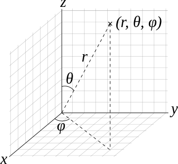
So the volume element spanning from \(r\) to \(r+dr\) \(\theta\) to \(\theta + d\theta\), and \(\phi\) to \(\phi + d\phi\) is
\[\mathrm{d}V=r^2 \sin \theta \,\mathrm{d}r\,\mathrm{d}\theta\,\mathrm{d}\varphi.\]
The surface element spanning from\(\theta + d\theta\), and \(\phi\) to \(\phi + d\phi\) on a spherical surface at (constant) radius \(r\) is
\[ \mathrm{d}S_r=r^2\sin\theta\,\mathrm{d}\theta\,\mathrm{d}\varphi.\]
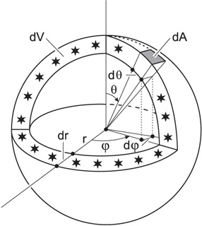
Surface area element dA and volume dV of a thin spherical shell, containing all the light sources at coordinate distance r.
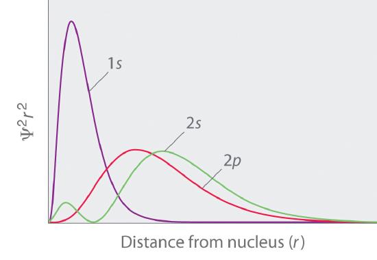
The quantity \(R(r)^* R(r)\) gives the radial probability density; i.e., the probability density for the electron to be at a point located the distance r from the proton. Radial probability densities for three types of atomic orbitals are plotted below.
When the radial probability density for every value of \(r\) is multiplied by the area of the spherical surface element (\(dS\) represented by that particular value of \(r\), we get the radial distribution function. The radial distribution function gives the probability density for an electron to be found anywhere on the surface of a sphere located a distance \(r\) from the proton. Since the area of a spherical surface is \(4 \pi r^2\), the radial distribution function is given by
\[\color{red} 4 \pi r^2 R(r)^* R(r)\]
Example: Most probable radius
Show that for a 1s orbital of a hydrogen-like atom the most probable distance from nucleus to electron is \(a_0/Z\).
- Solution
-
From the table in previous lecture:
\[ \begin{align*} \psi_{1s} &= \psi_{1,0,0}(r,\theta,\phi) \\[4pt] &= R_{1,0}(r)Y_{0,0}(\theta,\phi) \\[4pt] &= \dfrac{1}{\sqrt{\pi}}\left(\dfrac{Z}{a_0}\right)^{\frac{3}{2}}exp(-Zr/a_0) \end{align*}\]
where \(Z\) is the atomic number and \(a_0\) is the Bohr radius (\(5.29 \times 10^{-11} \,m\)).
The radial probability density for this state is:
\[ \color{red}{4 \pi r^2} \color{black}{ \psi_{1,0,0}^2} = 4\left(\dfrac{Z}{a_0}\right)^3\color{red}{r^2} \color{black}exp(-2Zr/a_0) \nonumber\]
Note to find the most probable distance from proton to electron, we take the derivative of the radial probability density and set to zero
\[\begin{align*} \dfrac{d}{dr} 4 \pi r^2\psi_{1,0,0}^2 &= \dfrac{d}{dr}\left[ 4 \left(\dfrac{Z}{a_0}\right)^3r^2exp(-2Zr/a_0)\right] = 0 \\[4pt] &= 4 \left(\dfrac{Z}{a_0}\right)^3 \left(2r - r^2 \dfrac{2Z}{a_0}\right )exp(-2Zr/a_0) =0 \end{align*} \]
This is established only when the polynomial term is zero (since the exponential and scalar factors will never be zero). So the radial probability density will be maximized when
\[2r- r^2 \dfrac{2Z}{a_0} = 0 \nonumber\]
Divide both sides by \(2r\) and solve for \(r\)
\[\begin{align*} 1- r\dfrac{Z}{a_0} &= 0 \\[4pt] r &= \dfrac{a_o}{Z} \end{align*}\]
Example: Probability
Calculate the probability of finding a 1s hydrogen electron being found within distance \(2a_o\) from the nucleus.
- Solution
-
Note the wavefunction of hydrogen 1s orbital which is
\[ψ_{100}= \dfrac{1}{\sqrt{π}} \left(\dfrac{1}{a_0}\right)^{3/2} e^{-\rho} \nonumber\]
with \(\rho=\dfrac{r}{a_0} \).
The probability of finding the electron within \(2a_0\) distance from the nucleus will be:
\[prob= \underbrace{\int_{0}^{\pi} \sin \theta \, d\theta}_{over\, \theta} \, \overbrace{ \dfrac{1}{\pi a_0^3} \int_{0}^{2a_0} r^2 e^{-2r/a_0} dr}^{over\, r} \, \underbrace{ \int_{0}^{2\pi} d\phi }_{over\, \phi } \nonumber\]
Since \(\int_0^{\pi} \sin \theta d\theta=2\) and \( \int_0^{2\pi} d\phi=2\pi\), we have
\[\begin{align*} prob &=2 \times 2\pi \times \dfrac{1}{\pi a_0^3} \int_0^2a_0 (-a_0/2)r^2 d e^{-2r/a_0} \\[4pt] &=\dfrac{4}{a_0^3}(-\dfrac{a_0}{2}) (r^2 e^{-2r/a_0} |_0^{2a_0} - \int_0^{2a_0} 2r e^{-2r/a_0} dr) \\[4pt] &= -\dfrac{2}{a_0^2} [(2a_0)^2 e^{-4}-0-2\int_0^{2a_0} r (-\dfrac{a_0}{2}) d e^{-2r/a_0} ] \\[4pt] &=-\dfrac{2}{a_0^2}4a_0^2 e^{-4} +\dfrac{4}{a_0^2}(-\dfrac{a_0}{2}) (r e^{-2r/a_0} |_0^{2a_0}-\int_0^{2a_0} e^{-2r/a_0} dr ) \\[4pt] &=-8e^{-4}-\dfrac{2}{a_0} \left[2a_0e^{-4}-0-(-\dfrac{a_0}{2})e^{-2r/a_0} |_0^{2a_0} \right] \\[4pt] &=-8e^{-4}-4e^{-4}-e^{2r/a_0} |_0^{2a_0} \\[4pt] &=-12 e^{-4}-(e^{-4}-1)=1-13e^{-4}=0.762 \end{align*}\]
There is a 76.2% probability that the electrons will be within \(2a_o\) of the nucleus in the 1s eigenstate.
The \(l\) Quantum number characterizes Angular Momentum and Angular Component (Ignoring the Radial Component)
As \(n\) increases the average value of \(r\) increases, which agrees with the fact that the energy of the electron also increases as \(n\) increases. The increased energy results in the electron being on the average pulled further away from the attractive force of the nucleus. As in the simple example of an electron moving on a line, nodes (values of \(r\) for which the electron density is zero) appear in the probability distributions. The number of nodes increases with increasing energy and equals \(n - 1\).
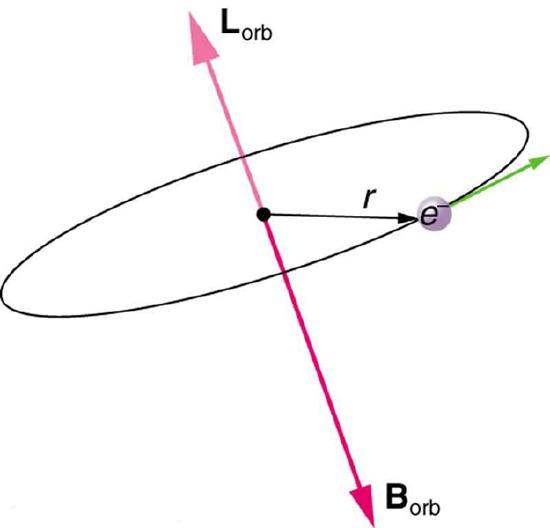
An electron possesses orbital angular momentum is the density distributions is no longer spherical.
The quantum number \(l\) governs the magnitude of the angular momentum, just as the quantum number \(n\) determines the energy. The magnitude of the angular momentum may assume only those values given by:
\[ |L| = \sqrt{l(l+1)} \hbar \label{4}\]
with \(l = 0, 1, 2, 3, ... n-1\).
When the electron possesses angular momentum the density distributions are no longer spherical. In fact for each value of \(\ell\), the electron density distribution assumes a characteristic shape Figure \(\PageIndex{6}\).
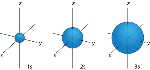
For any value of n, a value of \(\ell=0\) places that electron in an s orbital. This orbital is spherical in shape:
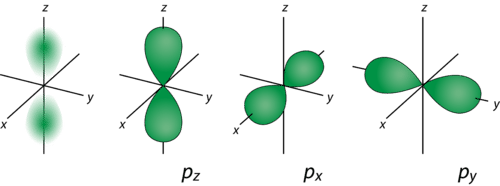
When \(\ell=1\) these are designated as p orbitals and have dumbbell shapes. Each of the p orbitals has a different orientation in three-dimensional space.
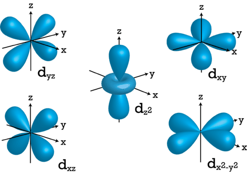
For \(\ell=2\), the \(m_l\) values can be -2, -1, 0, +1, +2 for a total of five d orbitals. Note that all five of the orbitals have specific three-dimensional orientations.
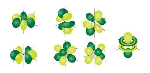
The most complex set of orbitals are the f orbitals. When \(\ell=3\), the \(m_l\) values can be -3, -2, -1, 0, +1, +2, +3 for a total of seven different orbital shapes. Again, note the specific orientations of the different f orbitals.
Exercise \(\PageIndex{1}\)
- For a Hydrogen atom what is the degeneracy for a specific \(n\) and \(l\)?
- Does that appear familiar?
- For a Hydrogen atom what is the degeneracy for a specific \(n\)?