
20: Variational Method Approximation and Linear Varational Method
- Page ID
- 198585

\( \newcommand{\vecs}[1]{\overset { \scriptstyle \rightharpoonup} {\mathbf{#1}} } \)
\( \newcommand{\vecd}[1]{\overset{-\!-\!\rightharpoonup}{\vphantom{a}\smash {#1}}} \)
\( \newcommand{\dsum}{\displaystyle\sum\limits} \)
\( \newcommand{\dint}{\displaystyle\int\limits} \)
\( \newcommand{\dlim}{\displaystyle\lim\limits} \)
\( \newcommand{\id}{\mathrm{id}}\) \( \newcommand{\Span}{\mathrm{span}}\)
( \newcommand{\kernel}{\mathrm{null}\,}\) \( \newcommand{\range}{\mathrm{range}\,}\)
\( \newcommand{\RealPart}{\mathrm{Re}}\) \( \newcommand{\ImaginaryPart}{\mathrm{Im}}\)
\( \newcommand{\Argument}{\mathrm{Arg}}\) \( \newcommand{\norm}[1]{\| #1 \|}\)
\( \newcommand{\inner}[2]{\langle #1, #2 \rangle}\)
\( \newcommand{\Span}{\mathrm{span}}\)
\( \newcommand{\id}{\mathrm{id}}\)
\( \newcommand{\Span}{\mathrm{span}}\)
\( \newcommand{\kernel}{\mathrm{null}\,}\)
\( \newcommand{\range}{\mathrm{range}\,}\)
\( \newcommand{\RealPart}{\mathrm{Re}}\)
\( \newcommand{\ImaginaryPart}{\mathrm{Im}}\)
\( \newcommand{\Argument}{\mathrm{Arg}}\)
\( \newcommand{\norm}[1]{\| #1 \|}\)
\( \newcommand{\inner}[2]{\langle #1, #2 \rangle}\)
\( \newcommand{\Span}{\mathrm{span}}\) \( \newcommand{\AA}{\unicode[.8,0]{x212B}}\)
\( \newcommand{\vectorA}[1]{\vec{#1}} % arrow\)
\( \newcommand{\vectorAt}[1]{\vec{\text{#1}}} % arrow\)
\( \newcommand{\vectorB}[1]{\overset { \scriptstyle \rightharpoonup} {\mathbf{#1}} } \)
\( \newcommand{\vectorC}[1]{\textbf{#1}} \)
\( \newcommand{\vectorD}[1]{\overrightarrow{#1}} \)
\( \newcommand{\vectorDt}[1]{\overrightarrow{\text{#1}}} \)
\( \newcommand{\vectE}[1]{\overset{-\!-\!\rightharpoonup}{\vphantom{a}\smash{\mathbf {#1}}}} \)
\( \newcommand{\vecs}[1]{\overset { \scriptstyle \rightharpoonup} {\mathbf{#1}} } \)
\(\newcommand{\longvect}{\overrightarrow}\)
\( \newcommand{\vecd}[1]{\overset{-\!-\!\rightharpoonup}{\vphantom{a}\smash {#1}}} \)
\(\newcommand{\avec}{\mathbf a}\) \(\newcommand{\bvec}{\mathbf b}\) \(\newcommand{\cvec}{\mathbf c}\) \(\newcommand{\dvec}{\mathbf d}\) \(\newcommand{\dtil}{\widetilde{\mathbf d}}\) \(\newcommand{\evec}{\mathbf e}\) \(\newcommand{\fvec}{\mathbf f}\) \(\newcommand{\nvec}{\mathbf n}\) \(\newcommand{\pvec}{\mathbf p}\) \(\newcommand{\qvec}{\mathbf q}\) \(\newcommand{\svec}{\mathbf s}\) \(\newcommand{\tvec}{\mathbf t}\) \(\newcommand{\uvec}{\mathbf u}\) \(\newcommand{\vvec}{\mathbf v}\) \(\newcommand{\wvec}{\mathbf w}\) \(\newcommand{\xvec}{\mathbf x}\) \(\newcommand{\yvec}{\mathbf y}\) \(\newcommand{\zvec}{\mathbf z}\) \(\newcommand{\rvec}{\mathbf r}\) \(\newcommand{\mvec}{\mathbf m}\) \(\newcommand{\zerovec}{\mathbf 0}\) \(\newcommand{\onevec}{\mathbf 1}\) \(\newcommand{\real}{\mathbb R}\) \(\newcommand{\twovec}[2]{\left[\begin{array}{r}#1 \\ #2 \end{array}\right]}\) \(\newcommand{\ctwovec}[2]{\left[\begin{array}{c}#1 \\ #2 \end{array}\right]}\) \(\newcommand{\threevec}[3]{\left[\begin{array}{r}#1 \\ #2 \\ #3 \end{array}\right]}\) \(\newcommand{\cthreevec}[3]{\left[\begin{array}{c}#1 \\ #2 \\ #3 \end{array}\right]}\) \(\newcommand{\fourvec}[4]{\left[\begin{array}{r}#1 \\ #2 \\ #3 \\ #4 \end{array}\right]}\) \(\newcommand{\cfourvec}[4]{\left[\begin{array}{c}#1 \\ #2 \\ #3 \\ #4 \end{array}\right]}\) \(\newcommand{\fivevec}[5]{\left[\begin{array}{r}#1 \\ #2 \\ #3 \\ #4 \\ #5 \\ \end{array}\right]}\) \(\newcommand{\cfivevec}[5]{\left[\begin{array}{c}#1 \\ #2 \\ #3 \\ #4 \\ #5 \\ \end{array}\right]}\) \(\newcommand{\mattwo}[4]{\left[\begin{array}{rr}#1 \amp #2 \\ #3 \amp #4 \\ \end{array}\right]}\) \(\newcommand{\laspan}[1]{\text{Span}\{#1\}}\) \(\newcommand{\bcal}{\cal B}\) \(\newcommand{\ccal}{\cal C}\) \(\newcommand{\scal}{\cal S}\) \(\newcommand{\wcal}{\cal W}\) \(\newcommand{\ecal}{\cal E}\) \(\newcommand{\coords}[2]{\left\{#1\right\}_{#2}}\) \(\newcommand{\gray}[1]{\color{gray}{#1}}\) \(\newcommand{\lgray}[1]{\color{lightgray}{#1}}\) \(\newcommand{\rank}{\operatorname{rank}}\) \(\newcommand{\row}{\text{Row}}\) \(\newcommand{\col}{\text{Col}}\) \(\renewcommand{\row}{\text{Row}}\) \(\newcommand{\nul}{\text{Nul}}\) \(\newcommand{\var}{\text{Var}}\) \(\newcommand{\corr}{\text{corr}}\) \(\newcommand{\len}[1]{\left|#1\right|}\) \(\newcommand{\bbar}{\overline{\bvec}}\) \(\newcommand{\bhat}{\widehat{\bvec}}\) \(\newcommand{\bperp}{\bvec^\perp}\) \(\newcommand{\xhat}{\widehat{\xvec}}\) \(\newcommand{\vhat}{\widehat{\vvec}}\) \(\newcommand{\uhat}{\widehat{\uvec}}\) \(\newcommand{\what}{\widehat{\wvec}}\) \(\newcommand{\Sighat}{\widehat{\Sigma}}\) \(\newcommand{\lt}{<}\) \(\newcommand{\gt}{>}\) \(\newcommand{\amp}{&}\) \(\definecolor{fillinmathshade}{gray}{0.9}\)Recap of Lecture 19
Last lecture address three aspects: (1) We continued to discussed the complications of electron-electron repulsions in solving Schrodinger equations of atomic systems and showed the "Ignorance is Bliss" approach is really pretty poor. (2) we discussed a qualitative way to address these repulsions by introducing an effective charge interpreted within a shielding and penetration perspective (this was discussed primarily within the context of radial distribution functions). (3) We motivated variational method by arguing the energy of a trial wavefunction will be lowest when it most likely resembles the true wavefunction (the same for the corresponding energies).
Approximations
The "ignorance is bliss" approximation
Ignore the \(\dfrac {e^2}{4\pi\epsilon_0 r_{12}}\) electron-electron repulsion term. This assume electron 1 is separable from electron 2, so that
\[\psi_{total} = \psi_{el_{1}}\psi_{el_{2}}\]
or in braket notation
\[ | \psi_{total} \rangle = \hat{H} | \psi_{el_1} \rangle | \psi_{el_2} \rangle\]
With some operator algebra, something important arises - the one electron energies are additive:
\[\hat{H} \psi_{total} = (\hat{H}_{el_1} + \hat{H}_{el_2}) \psi_{n\ {el_1}} \psi_{n\ {el_2}} = (E_{n_1} + E_{n_2}) \psi_{n\ {el_1}} \psi_{n\ {el_2}} \]
or in bra-ket notation
\[\hat{H} | \psi_{total} \rangle = \hat{H} | \psi_{el_1} \rangle | \psi_{el_2} \rangle = (E_{n_1} + E_{n_2}) | \psi_{1} \rangle | \psi_{1} \rangle \]
The energy for a ground state Helium atom (both electrons in lowest state) is then
\[E_{He_{1s}} = \underset{\text{energy of single electron in helium}}{E_{n_1}} + \underset{\text{energy of single electron in helium}}{E_{n_2}} = -R\left(\dfrac{Z^2}{1}\right) -R \left(\dfrac{Z^2}{1}\right) = -8R\]
where \(R\) is the Rydberg constant (\(13.6 \; eV\) that also maps the lowest energy of the hydrogen atom and \(Z=2\) for the helium nucleus. Experimentally, we find that the total energy for a ground state Helium atom \(E_{He_{1s}} = -5.8066\,R\). The big difference in results is due to the approximation we used to get to the value of \(-8\;R\). The "ignorance is bliss" approximation overestimates the energy of the helium atom greatly; this is a poor approximation and we need to address electron-electron repulsion properly (or better at least).
The general form of the "Ignorance is Bliss" approximation which almost as wrong as you can be for multi-electron atoms
\[\underbrace{E_{z} = nZ^2E_{z=1}}_{\text{bad approximation}}\]
Electron-electron repulsion results in "Shielding" -Redux
One way to take electron-electron repulsion into account is to modify the form of the wavefunction. A logical modification is to change the nuclear charge, \(Z\), in the wavefunctions to an effective nuclear charge, from +2 to a smaller value, \(Z_{eff}=\zeta\). The rationale for making this modification is that one electron partially shields the nuclear charge from the other electron.
Figure: Electron-electron shielding leads to a reduced effective nuclear charge. The attractive force of the nucleus on electron 2,\(V(r_2)\), is partially countered by the repulsive force between electron 1 and electron 2, \(V(r_{12})\).
Electron-electron shielding leads to a reduced effective nuclear charge. \(Z_{eff}\) is used instead of \(Z\) in radial part of wavefunctions.
A region of negative charge density between one of the electrons and the +2 nucleus makes the potential energy between them more positive (decreases the attraction between them). We can effect this change mathematically by using \(Z_{eff} < 2\) in the wavefunction expression. If the shielding were complete, then \(Z_{eff}\) would equal 1. If there is no shielding, then \(Z_{eff} = 2\). So a way to take into account the electron-electron interaction is by saying it produces a shielding effect. The shielding is not zero, and it isn't complete, so the effective nuclear charge is between one and two.
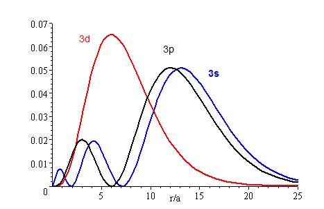
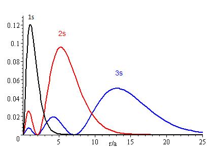
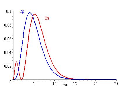
The lower the energy level, the higher the probability of finding the electron close to the nucleus. Also, the lower momentum quantum number gets, the closer it is to the nucleus.
The presence of \(Z_{eff}\) in the radial portions of the wavefunctions also means that the electron probability distributions associated with hydrogenic atomic orbitals in multi-electron systems are different from the exact atomic orbitals for hydrogen. The Figure above compares the radial distribution functions for an electron in a 1s orbital of hydrogen (the ground state), a 2s orbital in hydrogen (an excited configuration of hydrogen) and a 1s orbital in helium that is described by the best variational value of \(Z_{eff}\). Our use of hydrogen-like orbitals in quantum mechanical calculations for multi-electron atoms helps us to interpret our results for multi-electron atoms in terms of the properties of a system we can solve exactly.
Shielding is like a Nickelback concert
More electrons create the shielding or screening effect. Shielding or screening means the electrons closer to the nucleus block the outer valence electrons from getting close to the nucleus.

Imagine being in a crowded auditorium in a Nickelback concert. The enthusiastic fans are going to surround the auditorium, trying to get as close to the celebrity on the stage as possible. They are going to prevent people in the back from seeing the celebrity or even the stage. This is shielding. The stage is the nucleus and the celebrity is the protons. The fans are the electrons. Electrons closest to the nucleus will try to be as close to the nucleus as possible. The outer/valence electrons that are farther away from the nucleus will be shielded by the inner electrons. Therefore, the inner electrons prevent the outer electrons from forming a strong attraction to the nucleus. The degree to which the electrons are being screened by inner electrons can be shown by ns<np<nd<nf where n is the energy level. The inner electrons will be attracted to the nucleus much more than the outer electrons. Thus, the attractive forces of the valence electrons to the nucleus are reduced due to the shielding effects. That is why it is easier to remove valence electrons than the inner electrons. It also reduces the nuclear charge of an atom.
Penetration
Penetration is the ability of an electron to get close to the nucleus. Thus, the closer the electron is to the nucleus, the higher the penetration. Electrons with higher penetration will shield outer electrons from the nucleus more effectively. Electrons with higher penetration are closer to the nucleus than electrons with lower penetration. Electrons with lower penetration are being shielded from the nucleus more.
Slater's Rules Crudely Approximate Shielding
Slater's rules are an old and not-unreasonable way to estimate the effective nuclear charge \(Z_{eff}\) from the real number of protons in the nucleus and the effective shielding of electrons in each orbital "shell" (e.g., to compare the effective nuclear charge and shielding 3d and 4s in transition metals). The proper approach requires solving the Schrödinger equations (e.g., in the variational method), but this is a good rule of thumb that illustrates the gist.
- Step 1: Write the electron configuration of the atom in the following form:
(1s) (2s, 2p) (3s, 3p) (3d) (4s, 4p) (4d) (4f) (5s, 5p) . . .
- Step 2: Identify the electron of interest, and ignore all electrons in higher groups (to the right in the list from Step 1). These do not shield electrons in lower groups
- Step 3: Slater's Rules is now broken into two cases:
- the shielding experienced by an s- or p- electron, and
- the shielding experienced by a d- or f- electron.
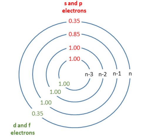
Graphical depiction of Slater's rules with shielding constants indicated.
| Group | Other electrons in the same group | Electrons in group(s) with principal quantum number n and azimuthal quantum number < l | Electrons in group(s) with principal quantum number n-1 | Electrons in all group(s) with principal quantum number < n-1 |
|---|---|---|---|---|
| [1s] | 0.30 | - | - | - |
| [ns,np] | 0.35 | - | 0.85 | 1 |
| [nd] or [nf] | 0.35 | 1 | 1 | 1 |
Sum together the contributions as described in the appropriate rule above to obtain an estimate of the shielding constant, \(S\). S is found by totaling the screening by all electrons except the one in question.
\[ S = \sum n_i S_i \]
We can quantitatively represent this difference between \(Z\) and \(Z_{eff}\) as follows:
\[ S=Z-Z_{eff} \]
Rearranging this formula to solve for \(Z_{eff}\) we obtain:
\[ Z_{eff}=Z-S \]
For a more basic overview of shielding and orbital penetration, check this module out.
Example \(\PageIndex{1}\)
What is the shielding constant experienced by a 2p electron in the nitrogen atom?
- Strategy:
- Determine the electron configuration of nitrogen (Z=7), then write it in the appropriate form. Use the Slater Rules to calculate the shielding constant for the electron.
- Solution:
-
A N: 1s2 2s2 2p3
N: (1s2)(2s2,2p3)
B S[2p] = 1.00(0) + 0.85(2) + 0.35(4) = 3.10
Now, what is it effective charge?
- Effective Charge:
-
\[ Z_{eff}=Z-S \]
\[ Z_{eff} = 7 - 3.10 = 3.9\]
Now, what is it effective energy of this electron if is followed the hydrogen atom energy (single electron system)?
- Effective Energy:
-
\(E_{2p}=-R\dfrac{Z^2}{n^2}\).
Let's substitute \(Z_{eff}\) for \(Z\) then
\[E_{2p}=-R \dfrac{Z_{Eff}^2}{n^2}\]
\[E_{2p} = - R \dfrac{(3.10)^2}{2^2} \approx -2.4R\]
Slaters rules provide an approximate guide to explain why certain orbitals fill before others since electrons in different orbitals will have a different effective nuclear charge due to different shielding resulting in differing energy levels.
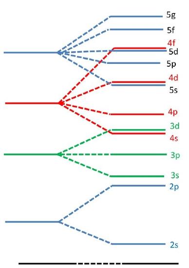
(left) This energy levels for a hydrogen atom (the degeneracy per level is \(n^2\)). (right) The energy levels for a multi-electron atom (the \(\ell\) degeneracy is broken, but not the \(m_l\) degeneracy.
The Variational Method Approximation
Start with the lowest energy state of a system \(\psi_0\). For the hydrogen atom, this state is \(\psi_{100}\), for the Harmonic Oscillator this state is \(v=0\), and for the Rigid Rotor this state is \(J=0\). Variational theorem states that if you substitute any function \(\phi\) for the true wavefunction \(\psi_0\), then calculate
\[ \color{red} E_{\phi} = \dfrac {\displaystyle \int \phi^* \hat{H} \phi d\tau}{\displaystyle \int \phi^* \phi d\tau} \ge E_o \label{1a}\]
where \(E_0\) is the true energy of the system. Equation \(\ref{1a}\) in braket notation is
\[ \color{red}E_{\phi} = \dfrac { \langle \phi | \hat{H} | \phi \rangle} { \langle \phi | \phi \rangle} \ge E_o \label{1b}\]
Note that \(E_{\phi} = E_0\) when \(\psi_0 = \phi\). This means that we can use any \(\phi\) and we will find \(E_{\phi}\), which is an upper bound for \(E_0\). The closer \(\phi\) is to \(\psi_0\), the lower the value of \(E_{\phi}\). The minimization of \(E_{\phi}\) leads to a better estimate of \(E_0\) and \(\psi_0\). Set \(\phi(\alpha,\beta,\gamma)\) with adjustable parameters \(\alpha, \beta, \gamma\), and solve for the parameters by differentiating \(E_{\phi}\) with respect to each parameter and setting the derivatives in equal to 0. In formulas,
\[\dfrac {dE_{\phi}}{d\alpha} = 0, \label{2a}\]
\[\dfrac {dE_{\phi}}{d\beta}=0 \label{2b}\]
\[\dfrac {dE_{\phi}}{d\gamma}=0\label{2c}\]
Equation \(\ref{1b}\) is call the variational theorem and states that for a time-independent Hamiltonian operator, any trial wave function will have an variational energy expectation value that is greater than or equal to the true ground state wave function corresponding to the given Hamiltonian. Because of this, the variational energy is an upper bound to the true ground state energy of a given molecule.
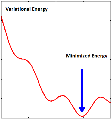
The optimum parameters in a trial wavefunction are found by searching for minima in the potential landscape spanned by those parameters
The general approach of this method consists in choosing a "trial wavefunction" depending on one or more parameters, and finding the values of these parameters for which the expectation value of the energy is the lowest possible (Figure \(\PageIndex{2}\)).
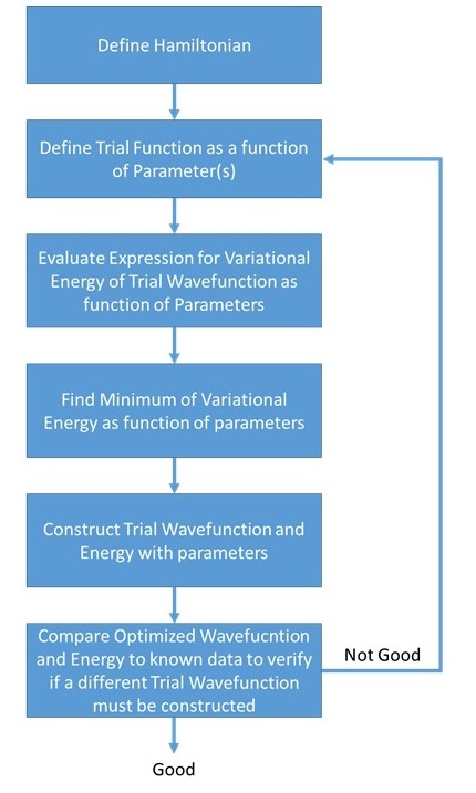
As is clear from Equations \ref{2a}-\ref{2c}, the variational method approximation requires that a trial wavefunction with one or more adjustable parameters be chosen.
Applying Variational Method to a Helium Atom
Conceptually, the Hamiltonian for Helium atom consists of the kinetic energy for electron 1 and electron 2, the electron-nucleus attraction, and the electron-electron repulsion.
\[\hat{H} = -\dfrac {\hbar^2}{2m_e} \left(\bigtriangledown_1^2 + \bigtriangledown_2^2\right) - \dfrac {Ze^2}{4\pi \epsilon_0} \left(\dfrac {1}{r_1} + \dfrac {1}{r_2} \right) + \dfrac {e^2}{4\pi\epsilon_0 r_{12}}\label{3}\]
Rearranging this equation gives the Hamiltonian in two one-electron equations and one repulsion term.
\[\hat{H} = \underbrace{\dfrac{-\hbar^2}{2m_e}\bigtriangledown_1^2 - \dfrac {Ze^2}{4\pi\epsilon_0 r_1}}_{\text{electron 1 in Hydrogen Orbital with Z=2}} + \underbrace { \dfrac {-\hbar^2}{2m_e}\bigtriangledown_2^2 - \dfrac {Ze^2}{4\pi\epsilon_0 r_2}}_{\text{electron 2 in Hydrogen Orbital with Z=2}} + \underbrace{\dfrac {e^2}{4\pi\epsilon_0 r_{12}}}_{\text{annoying electron-electron repulsion}} \label{4}\]
We use \(\psi_{H_{1s}}\) as our wave function \(\psi_0\). Then we define our trial wavefunction
\[\phi(r_1,r_2) = \psi_{H_{1s}}(r_1)\psi_{H_{1s}}(r_2)\]
and set \(\zeta\) as the adjustable parameter.
This is sort of like the "Ignorance is Bliss" approximation, but with \(\zeta\) that is varied to handle sheilding and better describe the true wavefunction.
The general idea is that the electron-electron repulsion has the effect of reducing shielding, the effective positive charge of the nucleus. The energy of this trial wavefunction as function of \(Z_{eff} \approx \zeta\) is evaluated to be
\[E_{trial}(\zeta) = \dfrac {m_e e^4}{16\pi^2 \epsilon_0^2 \hbar^2} \left(\zeta^2 - \dfrac {27}{8}\zeta \right)\label{5}\]
Upon taking the derivative with respect to \(\zeta\) setting the derivative equal to \(0\)
\[ \left. \dfrac{d E_{trial}(\zeta) }{ d \zeta}\right |_{\zeta_{min}} = 0\]
gives a minima at
\[\zeta_{min} = \dfrac {27}{16} \approx 1.69.\]
For an unshielded helium system, the expected \(\zeta\) should have a value of two
\[ \zeta_{min} = Z = 2\]
This is the origin of the shielding concept.
According to the variation principle, the minimum value of the energy on this graph is the best approximation of the true energy of the two-electron helium system, and the associated value of \(\zeta\) is the best value for the adjustable parameter.
Using the mathematical function for the energy of a system, the minimum energy with respect to the adjustable parameter can be found by taking the derivative of the energy with respect to that parameter, setting the resulting expression equal to zero, and solving for the parameter, in this case \(\zeta\).
How do you know when you are correct (i.e., the trial function looks like the real wavefunction when minimized for energy)?
You do not from the theory alone, but you can get that information from comparing to experiment.
When this procedure is carried out for the He atom with \(Z=2\), we find \(\zeta_{min} = 1.6875\) and the approximate energy (Equation \ref{5}) we calculate using this optimized paramter is
\[E \approx = -77.483\; eV.\]
Table shows that a substantial improvement in the accuracy of the computed binding energy is obtained by using shielding to account for the electron-electron interaction. Including the effect of electron shielding in the wavefunction reduces the error in the binding energy to about 2%. This idea is very simple, elegant, and significant.
|
|
|
|
|---|---|---|
|
|
|
-3.9983266 |
|
|
|
-2.84744797 |
|
|
|
-2.9032 |
Helium Atom Examples
We can choose any trail wavefunction we like for the Variational method. The closer the trial function looks like the real wavefunction (Solution to the unsolvable, by us at least, Schrödinger equation), the lower its energy will be.
First Trial Wavefunction
A logical first choice for such a function would be to assume that the electrons in the helium atom occupy two identical, but scaled, hydrogen 1s orbitals.
\[ | \psi (1,2) \rangle = | \phi (1) \phi (2) \rangle \label{orbital1}\]
with
- \(| \phi (1) = \exp(- \alpha r_1) \)
- \(| \phi (2)= \exp(- \alpha r_2) \).
The wavefunction in Equation \ref{orbital1} can the simplified:
\[ \begin{align}| \psi (1,2) \rangle &= | \phi (1) \phi (2) \rangle \\[4pt] &= \exp(- \alpha r_1) \exp(- \alpha r_2) \\[4pt] &= \exp\left[- \alpha (r_1 +r_2)\right] \label{7.3.2}\end{align}\]
The variational energy is determined by \(\langle \psi (1,2) | \hat{H} | \psi (1,2) \rangle\) with the Hamiltonian given by Equation \ref{3}. Minimizing this variable energy with respect to \(\alpha\) gives
\[E = -2.84766 \;E_h\]
which can be compared to the experimental value
\[ \left| \dfrac{E(\alpha)-E_{\exp}}{E_{\exp}} \right| = \left| \dfrac{-2.84766 \;E_h + 2.90372 \;E_h}{-2.90372 \;E_h} \right| = 1.93 \%\]
Second Trial Wavefunction
Some electron correlation can be built into the wavefunction by assuming that each electron is in an orbital that is a linear combination of two different and scaled hydrogen 1s orbitals.
\[| \psi (1,2) \rangle = | \phi (1) \phi (2) \rangle \label{orbital2}\]
with
- \(| \phi (1) = \exp(- \alpha r_1) + \exp(- \beta r_1)\)
- \(| \phi (2)= \exp(- \alpha r_2) + \exp(- \beta r_2)\).
The wavefunction in Equation \ref{orbital2} can the exapnded:
\[\begin{align}| \psi (1,2) \rangle &= | \phi (1) \phi (2) \rangle \\[4pt] &= {\exp(- \alpha r_1 )\exp(- \alpha r_2)}+\exp(- \alpha r_1 )\exp(- \beta r_2)+\exp(- \beta r_1 )\exp(- \alpha r_2 )+\exp(- \beta r_1 )\exp(- \beta r_2 ) \label{7.3.4b} \end{align}\]
The variational energy is determined by \(\langle \psi (1,2) | \hat{H} | \psi (1,2) \rangle\) with the Hamiltonian given by Equation \ref{3}. Minimizing this variable energy with respect to \(\alpha\) and \(\beta\) gives
\[E =-2.86035 \;E_h\]
Deviation from experimental value:
\[ \left| \dfrac{E(\alpha)-E_{\exp}}{E_{\exp}} \right| = \left| \dfrac{-2.86035 \;E_h + 2.90372 \;E_h}{-2.90372 \;E_h} \right| = 1.49 \%\]
Third Trial Wavefunction
The extent of electron correlation can be increased further by eliminating the first and last term in the second wavefunction (Equation \(\ref{7.3.4b}\)). This yields a wavefunction of the form,
\[ | \psi (1,2) \rangle = \exp(- \alpha r_1 )\exp(- \beta r_2 ) + \exp(- \beta r_1 )\exp(- \alpha r_2 ) \label{7.3.5} \]
This trial wavefunction places the electrons in different scaled hydrogen 1s orbitals 100% of the time this adds further improvement in the agreement with the literature value of the ground state energy is obtained. This result is within 1% of the actual ground state energy of the helium atom.
The variational energy is determined by \(\langle \psi (1,2) | \hat{H} | \psi (1,2) \rangle\) with the Hamiltonian given by Equation \ref{3}. Minimizing this variable energy with respect to \(\alpha\) and \(\beta\) gives
\[E = -2.87566 \;E_h\]
Deviation from experimental value:
\[ \left| \dfrac{E(\alpha)-E_{\exp}}{E_{\exp}} \right| = \left| \dfrac{-2.87566 \;E_h + 2.90372 \;E_h}{-2.90372 \;E_h} \right| = 0.97 \%\]
Fourth Trial Wavefunction
The third trial wavefunction, however, still rests on the orbital approximation and, therefore, does not treat electron correlation adequately. Hylleraas took the calculation a step further by introducing electron correlation directly into the first trial wavefunction by adding a term, \(r_{12}\), involving the inter-electron separation.
\[| \psi (1,2) \rangle = \left(\exp[- \alpha ( r_1 + r_2 )]\right) \left(1 + \beta r_{12} \right) \label{7.3.6} \]
Now, if the electrons are far apart, then \(r_{12}\) is large and the magnitude of the wave function increases favors that configuration.
The variational energy is determined by \(\langle \psi (1,2) | \hat{H} | \psi (1,2) \rangle\) with the Hamiltonian given by Equation \ref{3}. Minimizing this variable energy with respect to \(\alpha\) and \(\beta\) gives
\[E = - 2.89112\; E_h\]
This modification of the trial wavefunction has further improved the agreement between theory and experiment to within 0.5%. Deviation from experimental value:
\[ \left| \dfrac{E(\alpha)-E_{\exp}}{E_{\exp}} \right| = \left| \dfrac{- 2.89112 \;E_h + 2.90372 \;E_h}{-2.90372 \;E_h} \right| = 0.43 \%\]
Fifth Trial Wavefunction
Chandrasakar brought about further improvement by adding Hylleraas's \(r_{12}\) term to the third trial wave function (Equation \(\ref{7.3.5}\)) as shown here.
\[| \psi (1,2) \rangle = \left[\exp(- \alpha r_1 )\exp(- \beta r_2 ) + \exp(- \beta r_1 )\exp(- \alpha r_2 ) \right][1 + \gamma r _{12} ] \label{7.3.7}\]
The variational energy is determined by \(\langle \psi (1,2) | \hat{H} | \psi (1,2) \rangle\) with the Hamiltonian given by Equation \ref{3}. Minimizing this variable energy with respect to \(\alpha\), \(\beta\), and \(\gamma\) gives
\[E = -2.90143 \;E_h\]
Deviation from experimental value is
\[ \left| \dfrac{E(\alpha)-E_{\exp}}{E_{\exp}} \right| = \left| \dfrac{E(\alpha)--2.90372 \;E_h}{-2.90372 \;E_h} \right| = 0.0789 \%\]