21: Linear Variational Theory
- Page ID
- 198586
\( \newcommand{\vecs}[1]{\overset { \scriptstyle \rightharpoonup} {\mathbf{#1}} } \)
\( \newcommand{\vecd}[1]{\overset{-\!-\!\rightharpoonup}{\vphantom{a}\smash {#1}}} \)
\( \newcommand{\dsum}{\displaystyle\sum\limits} \)
\( \newcommand{\dint}{\displaystyle\int\limits} \)
\( \newcommand{\dlim}{\displaystyle\lim\limits} \)
\( \newcommand{\id}{\mathrm{id}}\) \( \newcommand{\Span}{\mathrm{span}}\)
( \newcommand{\kernel}{\mathrm{null}\,}\) \( \newcommand{\range}{\mathrm{range}\,}\)
\( \newcommand{\RealPart}{\mathrm{Re}}\) \( \newcommand{\ImaginaryPart}{\mathrm{Im}}\)
\( \newcommand{\Argument}{\mathrm{Arg}}\) \( \newcommand{\norm}[1]{\| #1 \|}\)
\( \newcommand{\inner}[2]{\langle #1, #2 \rangle}\)
\( \newcommand{\Span}{\mathrm{span}}\)
\( \newcommand{\id}{\mathrm{id}}\)
\( \newcommand{\Span}{\mathrm{span}}\)
\( \newcommand{\kernel}{\mathrm{null}\,}\)
\( \newcommand{\range}{\mathrm{range}\,}\)
\( \newcommand{\RealPart}{\mathrm{Re}}\)
\( \newcommand{\ImaginaryPart}{\mathrm{Im}}\)
\( \newcommand{\Argument}{\mathrm{Arg}}\)
\( \newcommand{\norm}[1]{\| #1 \|}\)
\( \newcommand{\inner}[2]{\langle #1, #2 \rangle}\)
\( \newcommand{\Span}{\mathrm{span}}\) \( \newcommand{\AA}{\unicode[.8,0]{x212B}}\)
\( \newcommand{\vectorA}[1]{\vec{#1}} % arrow\)
\( \newcommand{\vectorAt}[1]{\vec{\text{#1}}} % arrow\)
\( \newcommand{\vectorB}[1]{\overset { \scriptstyle \rightharpoonup} {\mathbf{#1}} } \)
\( \newcommand{\vectorC}[1]{\textbf{#1}} \)
\( \newcommand{\vectorD}[1]{\overrightarrow{#1}} \)
\( \newcommand{\vectorDt}[1]{\overrightarrow{\text{#1}}} \)
\( \newcommand{\vectE}[1]{\overset{-\!-\!\rightharpoonup}{\vphantom{a}\smash{\mathbf {#1}}}} \)
\( \newcommand{\vecs}[1]{\overset { \scriptstyle \rightharpoonup} {\mathbf{#1}} } \)
\(\newcommand{\longvect}{\overrightarrow}\)
\( \newcommand{\vecd}[1]{\overset{-\!-\!\rightharpoonup}{\vphantom{a}\smash {#1}}} \)
\(\newcommand{\avec}{\mathbf a}\) \(\newcommand{\bvec}{\mathbf b}\) \(\newcommand{\cvec}{\mathbf c}\) \(\newcommand{\dvec}{\mathbf d}\) \(\newcommand{\dtil}{\widetilde{\mathbf d}}\) \(\newcommand{\evec}{\mathbf e}\) \(\newcommand{\fvec}{\mathbf f}\) \(\newcommand{\nvec}{\mathbf n}\) \(\newcommand{\pvec}{\mathbf p}\) \(\newcommand{\qvec}{\mathbf q}\) \(\newcommand{\svec}{\mathbf s}\) \(\newcommand{\tvec}{\mathbf t}\) \(\newcommand{\uvec}{\mathbf u}\) \(\newcommand{\vvec}{\mathbf v}\) \(\newcommand{\wvec}{\mathbf w}\) \(\newcommand{\xvec}{\mathbf x}\) \(\newcommand{\yvec}{\mathbf y}\) \(\newcommand{\zvec}{\mathbf z}\) \(\newcommand{\rvec}{\mathbf r}\) \(\newcommand{\mvec}{\mathbf m}\) \(\newcommand{\zerovec}{\mathbf 0}\) \(\newcommand{\onevec}{\mathbf 1}\) \(\newcommand{\real}{\mathbb R}\) \(\newcommand{\twovec}[2]{\left[\begin{array}{r}#1 \\ #2 \end{array}\right]}\) \(\newcommand{\ctwovec}[2]{\left[\begin{array}{c}#1 \\ #2 \end{array}\right]}\) \(\newcommand{\threevec}[3]{\left[\begin{array}{r}#1 \\ #2 \\ #3 \end{array}\right]}\) \(\newcommand{\cthreevec}[3]{\left[\begin{array}{c}#1 \\ #2 \\ #3 \end{array}\right]}\) \(\newcommand{\fourvec}[4]{\left[\begin{array}{r}#1 \\ #2 \\ #3 \\ #4 \end{array}\right]}\) \(\newcommand{\cfourvec}[4]{\left[\begin{array}{c}#1 \\ #2 \\ #3 \\ #4 \end{array}\right]}\) \(\newcommand{\fivevec}[5]{\left[\begin{array}{r}#1 \\ #2 \\ #3 \\ #4 \\ #5 \\ \end{array}\right]}\) \(\newcommand{\cfivevec}[5]{\left[\begin{array}{c}#1 \\ #2 \\ #3 \\ #4 \\ #5 \\ \end{array}\right]}\) \(\newcommand{\mattwo}[4]{\left[\begin{array}{rr}#1 \amp #2 \\ #3 \amp #4 \\ \end{array}\right]}\) \(\newcommand{\laspan}[1]{\text{Span}\{#1\}}\) \(\newcommand{\bcal}{\cal B}\) \(\newcommand{\ccal}{\cal C}\) \(\newcommand{\scal}{\cal S}\) \(\newcommand{\wcal}{\cal W}\) \(\newcommand{\ecal}{\cal E}\) \(\newcommand{\coords}[2]{\left\{#1\right\}_{#2}}\) \(\newcommand{\gray}[1]{\color{gray}{#1}}\) \(\newcommand{\lgray}[1]{\color{lightgray}{#1}}\) \(\newcommand{\rank}{\operatorname{rank}}\) \(\newcommand{\row}{\text{Row}}\) \(\newcommand{\col}{\text{Col}}\) \(\renewcommand{\row}{\text{Row}}\) \(\newcommand{\nul}{\text{Nul}}\) \(\newcommand{\var}{\text{Var}}\) \(\newcommand{\corr}{\text{corr}}\) \(\newcommand{\len}[1]{\left|#1\right|}\) \(\newcommand{\bbar}{\overline{\bvec}}\) \(\newcommand{\bhat}{\widehat{\bvec}}\) \(\newcommand{\bperp}{\bvec^\perp}\) \(\newcommand{\xhat}{\widehat{\xvec}}\) \(\newcommand{\vhat}{\widehat{\vvec}}\) \(\newcommand{\uhat}{\widehat{\uvec}}\) \(\newcommand{\what}{\widehat{\wvec}}\) \(\newcommand{\Sighat}{\widehat{\Sigma}}\) \(\newcommand{\lt}{<}\) \(\newcommand{\gt}{>}\) \(\newcommand{\amp}{&}\) \(\definecolor{fillinmathshade}{gray}{0.9}\)Recap of Lecture 20
Last lecture continued the discussion of variational method approach to approximate the solutions of systems that we cannot analytically solve the Schrodinger equation. The system that motivates us is multi-electron atoms, and we focused on the He atom primarily. This approach requires postulating a trial wavefunction and then calculating the energy of that function as a function of the parameters that describe the trial wavefunction. Then we can minimize the energy as a function of these parameters and the closer the wavefunction "looks" like the true wavefunction (that we do not know), the closer the trail energy matches the true energy (however, the trial energy is ALWAYS higher in energy than the true energy). We went over several example trial wavefunctions for the He atom showing the more complex wavefunctions give better results than the simple ones (including the "Ignorance is Bliss" approximation with an average effective charge). We then transition into the Heisenberg's matrix representation of Quantum mechanics which was the segway to the linear variational method, which addresses trial functions that are a linear combination of a basis functions. We will continue that discussed next lecture.
Overview (again) of Variational Method Approximation
We can always construct a variational energy for a trial wavefunction given a specific Hamilitonian
\[E_{trial} = \dfrac{\langle \psi_{trial}| \hat{H} | \psi_{trial} \rangle }{\langle \psi_{trial}| \psi_{trial} \rangle} \ge E_{true}\label{7.3.1b}\]
The variational energy is an upper bound to the true ground state energy of a given molecule. The general approach of this method consists in choosing a "trial wavefunction" depending on one or more parameters, and finding the values of these parameters for which the expectation value of the energy is the lowest possible.

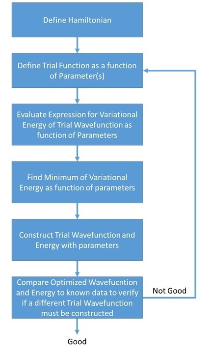
Simplified algorithmic flowchart of the Variational Method approximation
Example \(\PageIndex{1}\)
Using the variational method approximation, find the ground state energy of a particle in a box using this trial function:
\[| \phi \rangle = N\cos\left(\dfrac{\pi x}{L}\right) \nonumber \]
How does is it compare to the true ground state energy?
- Solution
-
The problem asks that we apply variational methods approximation to our trial wavefunction.
\[ E_{\phi} = \dfrac {\langle \phi | \hat{H} | \phi \rangle} { \langle \phi | \phi \rangle} \ge E_o \nonumber \]
Let's look at the denominator:
\[\langle \phi | \phi \rangle = 1 = \int_{0}^{L}N^2\cos^2\Big(\dfrac{\pi x}{L}\Big)\nonumber \]
Performing this integral and solving for N yields
\[N = \sqrt{\dfrac{2}{L}}\nonumber \]
Now let's look at the numerator:
The Hamiltonian for a particle in a one dimensional box is \(\hat{H} = \dfrac{-\hbar^2}{2m}\dfrac{d^2}{dx^2}\)
\[ \begin{align*} \langle \phi | \hat{H} | \phi \rangle &= \langle N\cos\Big(\dfrac{\pi x}{L}\Big) \Big| \dfrac{-\hbar^2}{2m}\dfrac{d^2}{dx^2} \Big| N\cos\Big(\dfrac{\pi x}{L}\Big) \rangle\nonumber \\ &= \int_{0}^{L}N\cos\Big(\dfrac{\pi x}{L}\Big)\dfrac{-\hbar^2}{2m}\dfrac{d^2}{dx^2}N\cos\Big(\dfrac{\pi x}{L}\Big)dx\nonumber \\ &= \dfrac{N^2\pi^2 \hbar^2}{2mL^2}\int_{0}^{L}\cos^2\Big(\dfrac{\pi x}{L}\Big) dx\end{align*} \]
where \(N = \sqrt{\dfrac{2}{L}}\). The above equation after the integral becomes
\[\dfrac{\pi^2 \hbar^2}{mL^3}\Big(\dfrac{L}{2}\Big)\nonumber \]
Now the variational energy for this trail wavefunction is
\[E_\phi = \dfrac{\pi^2 \hbar^2}{2mL^2}\nonumber \]
This is equal to the ground state energy of the particle in a box that we calculated from the Schrodinger equation using
\[\psi = \sqrt{\dfrac{2}{L}}\sin(\dfrac{n\pi x}{L})\nonumber \]
This is not a good trail wavefucntion since we are not varying any parameter, and moreover it is the eigenstate of energy. So the guess (trail wavefunction) is accurate... this almost never happens.
Let's look at a Different Type of a Trial Wavefunction
Let's expand \(\phi\) into a linear combination of basis functions:
\[ | \psi_{trial} \rangle = \sum_j^N a_j | \phi_j \rangle \label{Ex1}\]
and similarly
\[ \langle \psi_{trial} | = \sum_j^N a_j^* \langle \phi_j | \label{Ex2}\]
In these cases, one says that a 'linear variational' calculation is being performed.
Basis Functions
The set of functions {\(\phi_j\)} are called the 'linear variational' basis functions and are usually selected:
- to obey all of the boundary conditions that the exact state \(| \psi _{trial} \rangle\) obeys,
- to be functions of the the same coordinates as \(| \psi _{trial} \rangle\), and
- to be of the same symmetry as \(| \psi _{trial} \rangle\).
Beyond these conditions, the {\(\phi_j\)} are nothing more than members of a set of functions that are convenient to deal with (e.g., convenient to evaluate Hamiltonian terms elements \(\langle \phi_i|H|\phi_j \rangle\) that can, in principle, be made complete if more and more such functions are included in the expansion in Equations \(\ref{Ex1}\) and \(\ref{Ex2}\) (i.e., increase \(N\)).
Examples
For example, For the Hydrogen atom wavefunctions, \(\phi\) could be expanded into a linear combination of Scalable Gaussian functions
\[|\phi_{trial} \rangle = \sum_{j=1}^{N} c_{j} e^{-\alpha_{j} r^2}\label{6B}\]
or for \(H_2\), (this is call the Liner Combination of Atomic Orbitals approximation discussed in detail in later sections)
\[| \phi_{trial} \rangle = c_1 \psi_{1s_A} + c_2 \psi_{1s_B}\]
The goal is to solve for the set of all \(c\) values that minimize the energy \(E_{trial}\).
\[ E_{trial} = \dfrac{ \langle \psi _{trial}| \hat {H} | \psi _{trial} \rangle}{\langle \psi _{trial} | \psi _{trial} \rangle} \label{7.1.8}\]
Substituting Equation \ref{Ex2} into Equation \ref{7.1.8} involves addressing the numerator and denominator individually. For the numerator, the integral can be expanded thusly:
\[\begin{align} \langle\psi_{trial} |H| \psi_{trial} \rangle &= \sum_{i}^{N} \sum_{j} ^{N}a_i^{*} a_j \langle \phi_i|H|\phi_j \rangle. \\[5pt] &= \sum_{i,\,j} ^{N,\,N}a_i^{*} a_j \langle \phi_i|H|\phi_j \rangle. \label{MatrixElement}\end{align}\]
We often rewrite the following integral in Equation \ref{MatrixElement} (as a function of the basis elements, not the trial wavefunction) as
\[ H_{ij} = \langle \phi_i|H|\phi_j \rangle\]
So the numerator of the right side of Equation \ref{7.1.8} becomes
\[\langle\psi_{trial} |H| \psi_{trial} \rangle = \sum_{i,\,j} ^{N,\,N}a_i^{*} a_j H_{ij} \label{numerator}\]
Similarly, the denominator of the right side of Equation \ref{7.1.8} can be expanded
\[\langle \psi_{trial}|\psi_{trial} \rangle = \sum_{i,\,j} ^{N,\,N}a_i^{*} a_j \langle \phi_i | \phi_j \rangle \label{overlap}\]
We often rewrite the following integral in Equation \ref{overlap} (as a function of the basis elements, not the trial wavefunction) as
\[ S_{ij} = \langle \phi_i|\phi_j \rangle \]
where \(S_{ij}\) are overlap integrals between the different {\(\phi_j\)} functions. So Equation \ref{overlap} is
\[\langle \psi_{trial}|\psi_{trial} \rangle = \sum_{i,\,j} ^{N,\,N}a_i^{*} a_j S_{ij} \label{denominator}\]
Orthonormality
There is no explicit rule that the {\(\phi_j\)} functions have to be orthogonal and normal functions, although they often are selected that was for convenience. Therefore, a priori, \(S_{ij}\) does not have to be \(\delta_{ij}\).
Substituting Equations \ref{numerator} and \ref{denominator} into the variational energy formula (Equation \ref{7.1.8}) results in
\[ E_{trial} = \dfrac{ \displaystyle \sum_{i,\,j} ^{N,\,N}a_i^{*} a_j H_{ij} }{ \displaystyle \sum_{i,\,j} ^{N,\,N}a_i^{*} a_j S_{ij} } \label{Var}\]
Minimizing the Variational Energy
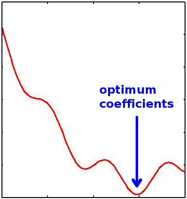
The optimum coefficients are found by searching for minima in the variational energy landscape spanned by varying the \(\{a_i\}\) coefficients (Figure \(\PageIndex{1}\)).

We want to minimize the variation energy with respect to the linear coefficients \(\{a_i\}\), which requires that
\[\dfrac{\partial E_{trial}}{\partial a_i}= 0\]
for all \(i\).
For the "normal" variational method discussed last time, the variation energy can be a nonlinear function of one or more parameters. Minimizing the variation energy therefore may require linear or non-linear regression. However, the linearatiy of the trial function and the nature of the variational energy allows for more simplistic linear regression.
The expression for variational energy (Equation \ref{Var}) can be rearranged
\[E_{trial} \sum_{i,\,j} ^{N,\,N} a_i^*a_j S_{ij} = \sum_{i,\,j} ^{N,\,N} a_i^* a_j H_{ij} \label{7.2.9}\]
Differentiating both sides of Equation \(\ref{7.2.9}\) for the \(k^{th}\) coefficient gives,
\[ \underbrace{ \dfrac{\partial E_{trial}}{\partial a_k} \sum_{i,\,j} ^{N,\,N} a_i^*a_j S_{ij}+ E_{trial} \sum_i \sum_j \left[ \dfrac{ \partial a_i^*}{\partial a_k} a_j + \dfrac {\partial a_j}{\partial c_k} a_i^* \right ]S_{ij} }_{\text{product rule}}= \sum_{i,\,j} ^{N,\,N} \left [ \dfrac{\partial a_i^*}{\partial a_k} a_j + \dfrac{ \partial a_j}{\partial a_k}a_i^* \right] H_{ij} \label{7.2.10}\]
Since the coefficients are linearly independent (Equation \ref{Ex1})
\[\dfrac{\partial a_i^*}{ \partial a_k} = \delta_{ik}\]
and
\[S_{ij}^* = S_{ji}\]
and also since the Hamiltonian is a Hermetian Operator
\[H_{ij}^* =H_{ji}\]
then Equation \(\ref{7.2.10}\) simplifies to
\[ \dfrac{\partial E_{trial}}{\partial a_k} \sum_i \sum_j a_i^*a_j S_{ij}+ 2E_{trial} \sum_i S_{ik} = 2 \sum_i a_i H_{ik} \label{7.2.11}\]
Hermitian Operators
Hermitian operators are operators that satisfy the general formula
\[ \langle \phi_i | \hat{A} | \phi_j \rangle = \langle \phi_j | \hat{A} | \phi_i \rangle \label{Herm1}\]
If that condition is met, then \(\hat{A}\) is a Hermitian operator. For any operator that generates a real eigenvalue (e.g., observables), then that operator is Hermitian. The Hamiltonian \(\hat{H}\) meets the condition and a Hermitian operator. Equation \ref{Herm1} can be rewriten as
\[A_{ij} =A_{ji}\]
where
\[A_{ij} = \langle \phi_i | \hat{A} | \phi_j \rangle\]
and
\[A_{ji} = \langle \phi_j | \hat{A} | \phi_i \rangle\]
Therefore, when applied to the Hamiltonian operator
\[\boxed{H_{ij}^* =H_{ji}.}\]
At the minimum variational energy, when
\[\dfrac{\partial E_{trial}}{\partial a_k} = 0\]
then Equation \(\ref{7.2.11}\) gives
\[ {\sum _i^N a_i (H_{ik}–E_{trial} S_{ik}) = 0} \label{7.2.12}\]
for all \(k\). The equations in \(\ref{7.2.12}\) are call the Secular Equations.


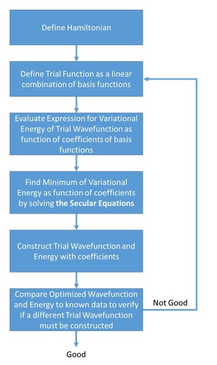
(left) Simplified algorithmic flowchart of the "normal" Variational Method approximation vs. (right) Simplified algorithmic flowchart of the linear Variational Method approximation. Noticed the similarities and differences between two.
Secular Determinant
From the secular equations with an orthonormal functions (Equation \ref{7.2.12}), we have \(k\) simultaneous secular equations in \(k\) unknowns. These equations can also be written in matrix notation, and for a non-trivial solution (i.e. \(c_i \neq 0\) for all \(i\)), the determinant of the secular matrix must be equal to zero.
\[ { | H–E_{trial}S| = 0} \label{7.2.13}\]
For a 3x3 system (i.e., expanded to three terms) Equation \ref{7.2.13} looks like:
\[\begin{vmatrix} H_{11}-E_{trial}S_{11}&H_{12}-E_{trial}S_{12} \\ H_{12}-E_{trial}S_{12}&H_{22}-E_{trial}S_{22}\end{vmatrix}=0\]
when the determinate is expanded, it will give a polynomial that will have N roots (solutions of E_{trials}).
Determinants OVerview
- The determinant is a real number, it is not a matrix.
- The determinant can be a negative number.
- It is not associated with absolute value at all except that they both use vertical lines.
- The determinant only exists for square matrices (2×2, 3×3, ... n×n). The determinant of a 1×1 matrix is that single value in the determinant.
- The inverse of a matrix will exist only if the determinant is not zero.
Determinants can be expanded using Minors and Cofactors
The method is called expansion using minors and cofactors. Before we can use them, we need to define them. It is the product of the elements on the main diagonal minus the product of the elements off the main diagonal.
In the case of a 2 × 2 matrix, the specific formula for the determinant is
\[{\displaystyle {\begin{aligned}|A|={\begin{vmatrix}a&b\\c&d\end{vmatrix}}=ad-bc.\end{aligned}}}\]
Similarly, suppose we have a 3 × 3 matrix A, and we want the specific formula for its determinant |A|:
\[{\displaystyle {\begin{aligned}|A|={\begin{vmatrix}a&b&c\\d&e&f\\g&h&i\end{vmatrix}}&=a\,{\begin{vmatrix}e&f\\h&i\end{vmatrix}}-b\,{\begin{vmatrix}d&f\\g&i\end{vmatrix}}+c\,{\begin{vmatrix}d&e\\g&h\end{vmatrix}}\\&=aei+bfg+cdh-ceg-bdi-afh.\end{aligned}}}\]
To solve this determinate in Equation \ref{7.2.13}, it should be expanded to generate a polynomial (a characteristic equation) that can be directly solved with linear methods (i.e., find the roots - different \(E_{trail}\) values that satisfy the secular equations).
Example \(\PageIndex{1}\): Optimizing a two-term basis set
If \(|\psi_{trial} \rangle\) is a linear combination of two functions. In math terms,
\[|\psi_{trial} \rangle= \sum_{n=1}^{N=2} a_n |f_n\rangle = a_1 |\phi_1 \rangle + a_2 | \phi_2 \rangle\]
then the secular determinant (Equation \(\ref{7.2.13}\)), in matrix formulation would look like this
\[\begin{vmatrix} H_{11}-E_{trial}S_{11}&H_{12}-E_{trial}S_{12} \\ H_{12}-E_{trial}S_{12}&H_{22}-E_{trial}S_{22}\end{vmatrix}=0\]
Solution
Solving the secular equations is done by finding \(E_{trial}\) and putting the value into the expansion of the secular determinant
\[a_1^2 H_{11} + 2a_1 a_2 H_{12}+ a_2^2 H_{22}=0\]
and
\[a_1(H_{12} - E_{trial}S_{12}) + a_2(H_{22} - E_{trial}S_{22}) = 0\]
Equation \(\ref{7.2.13}\) can be solved to obtain the energies \(E\). When arranged in order of increasing energy, these provide approximations to the energies of the first \(k\) states (each having an energy higher than the true energy of the state by virtue of the variation theorem). To find the energies of a larger number of states we simply use a greater number of basis functions \(\{\phi_i\}\) in the trial wavefunction (Example \ref{Ex1}). To obtain the approximate wavefunction for a particular state, we substitute the appropriate energy into the secular equations and solve for the coefficients \(a_i\).
Using this method it is possible to find all the coefficients \(a_1 \ldots a_k\) in terms of one coefficient; normalizing the wavefunction provides the absolute values for the coefficients.
Example: Polynomial Basis set for Approximating the Wavefunction of a Particle in an Infinite Potential Well
The potential well with infinite barriers is defined:
\[V(x) = \infty \;for | x| > |L|\]
and
\[V(x) = 0 \;for \; |x| \leq |L| \]
and it forces the wave function to vanish at the boundaries of the well at \(x=\pm a\). The exact solution for this problem is known and treated previously. Here we discuss a linear variational approach to be compared with the exact solution. We take \(a=1\) and use natural units such that \(\hbar^2/2m=1\).
As the all variational methods problems with a basis set, the trial wavefunction is expanded
\[| \varphi \rangle = \sum_n f_n(x) \]
As basis functions we take simple polynomials that vanish on the boundaries of the well:
\[ \psi_n(x)=x^n(x-1)(x+1)\]
with \(n=0,1,2,3...\)
The reason for choosing this particular form of basis functions is that the relevant matrix elements can easily be calculated analytically.
Solution
We start we the overlap matrix:
\[ S_{mn}=\langle \psi_n\vert\psi_m \rangle = \int_{-1}^1 \psi_n(x) \psi_m(x) dx.\]
Working out the integrals, one obtains
\[S_{mn}=\dfrac{2}{n+m+5} - \dfrac{4}{n+m+3} + \dfrac{2}{n+m+1}\]
for when \(n+m\) even, and zero otherwise.
We need to calculate the Hamiltonian matrix elements:
\[H_{mn}=\langle \psi_n \vert p^2 \vert \psi_m \rangle = \int_{-1}^1 \psi_n(x) \left(-\frac{d^2}{dx^2} \right) \psi_m(x) dx\]
\[ = -8 \left[ \dfrac{1-m-n-2mn} {(m+n+3)(m+n+1)(m+n-1)} \right] \]
for when \(n+m\) even, and zero otherwise.
Linear Combination of Trial Wavefunctions (e.g., Gaussian functions)
In electron calculations, the trial function approximation can be constructed in terms of the ground-state wavefunctions (remember that even the radial component of higher orbitals decay exponentially when far from the nucleus:
\[\phi = \sum_{j=1}^{N} c_j e^{-\alpha_j r}\label{10A}\]
An alternative to this trial wavefunction is the combination of Gaussian functions:
\[\phi = \sum_{j=1}^{N} c_j e^{-\alpha_j r^2}\label{10}\]
We know the energy of the hydrogen atom, but using a set of \(N\) Gaussian functions gives...
| \(N\) | \(E_{min}\) in Hartree units |
|---|---|
| 1 | -0.42441 |
| 2 | -0.48581 |
| 3 | -0.49697 |
| : | : |
| 5 | -0.49976 |
| : | : |
| 16 | -0.49998 |
A quick note on units - \(1 Hartree = 2 R_{\infty}\)
These sets of Gaussian functions are used in computer programs for molecular quantum mechanic calculations, because the integrals are much simpler than using the one-electron Hydrogen atomic functions. Besides, for multi-electron atoms, the H-atom functions are not as accurate.
Overview of Variational Methods
- The hyrogen atom is the only atom with an exact solution.
- Hydrogen wave functions are used as the approximation for atomic wave functions in multielectron atoms for atomic wavefunctions in multielectron atoms.
- The variational principle states that any wave function we choose that satisfies the Schrödinger equation will give an energy greater than the true energy of the system.
- The variation method provides a general prescription for improving on any wave function with a parameter by minimizing that function with respect to the parameter minimizing that function with respect to the parameter
Contributors
Michael Fowler (Beams Professor, Department of Physics, University of Virginia)


