Acid/Base Titrations
- Page ID
- 36197
\( \newcommand{\vecs}[1]{\overset { \scriptstyle \rightharpoonup} {\mathbf{#1}} } \)
\( \newcommand{\vecd}[1]{\overset{-\!-\!\rightharpoonup}{\vphantom{a}\smash {#1}}} \)
\( \newcommand{\dsum}{\displaystyle\sum\limits} \)
\( \newcommand{\dint}{\displaystyle\int\limits} \)
\( \newcommand{\dlim}{\displaystyle\lim\limits} \)
\( \newcommand{\id}{\mathrm{id}}\) \( \newcommand{\Span}{\mathrm{span}}\)
( \newcommand{\kernel}{\mathrm{null}\,}\) \( \newcommand{\range}{\mathrm{range}\,}\)
\( \newcommand{\RealPart}{\mathrm{Re}}\) \( \newcommand{\ImaginaryPart}{\mathrm{Im}}\)
\( \newcommand{\Argument}{\mathrm{Arg}}\) \( \newcommand{\norm}[1]{\| #1 \|}\)
\( \newcommand{\inner}[2]{\langle #1, #2 \rangle}\)
\( \newcommand{\Span}{\mathrm{span}}\)
\( \newcommand{\id}{\mathrm{id}}\)
\( \newcommand{\Span}{\mathrm{span}}\)
\( \newcommand{\kernel}{\mathrm{null}\,}\)
\( \newcommand{\range}{\mathrm{range}\,}\)
\( \newcommand{\RealPart}{\mathrm{Re}}\)
\( \newcommand{\ImaginaryPart}{\mathrm{Im}}\)
\( \newcommand{\Argument}{\mathrm{Arg}}\)
\( \newcommand{\norm}[1]{\| #1 \|}\)
\( \newcommand{\inner}[2]{\langle #1, #2 \rangle}\)
\( \newcommand{\Span}{\mathrm{span}}\) \( \newcommand{\AA}{\unicode[.8,0]{x212B}}\)
\( \newcommand{\vectorA}[1]{\vec{#1}} % arrow\)
\( \newcommand{\vectorAt}[1]{\vec{\text{#1}}} % arrow\)
\( \newcommand{\vectorB}[1]{\overset { \scriptstyle \rightharpoonup} {\mathbf{#1}} } \)
\( \newcommand{\vectorC}[1]{\textbf{#1}} \)
\( \newcommand{\vectorD}[1]{\overrightarrow{#1}} \)
\( \newcommand{\vectorDt}[1]{\overrightarrow{\text{#1}}} \)
\( \newcommand{\vectE}[1]{\overset{-\!-\!\rightharpoonup}{\vphantom{a}\smash{\mathbf {#1}}}} \)
\( \newcommand{\vecs}[1]{\overset { \scriptstyle \rightharpoonup} {\mathbf{#1}} } \)
\(\newcommand{\longvect}{\overrightarrow}\)
\( \newcommand{\vecd}[1]{\overset{-\!-\!\rightharpoonup}{\vphantom{a}\smash {#1}}} \)
\(\newcommand{\avec}{\mathbf a}\) \(\newcommand{\bvec}{\mathbf b}\) \(\newcommand{\cvec}{\mathbf c}\) \(\newcommand{\dvec}{\mathbf d}\) \(\newcommand{\dtil}{\widetilde{\mathbf d}}\) \(\newcommand{\evec}{\mathbf e}\) \(\newcommand{\fvec}{\mathbf f}\) \(\newcommand{\nvec}{\mathbf n}\) \(\newcommand{\pvec}{\mathbf p}\) \(\newcommand{\qvec}{\mathbf q}\) \(\newcommand{\svec}{\mathbf s}\) \(\newcommand{\tvec}{\mathbf t}\) \(\newcommand{\uvec}{\mathbf u}\) \(\newcommand{\vvec}{\mathbf v}\) \(\newcommand{\wvec}{\mathbf w}\) \(\newcommand{\xvec}{\mathbf x}\) \(\newcommand{\yvec}{\mathbf y}\) \(\newcommand{\zvec}{\mathbf z}\) \(\newcommand{\rvec}{\mathbf r}\) \(\newcommand{\mvec}{\mathbf m}\) \(\newcommand{\zerovec}{\mathbf 0}\) \(\newcommand{\onevec}{\mathbf 1}\) \(\newcommand{\real}{\mathbb R}\) \(\newcommand{\twovec}[2]{\left[\begin{array}{r}#1 \\ #2 \end{array}\right]}\) \(\newcommand{\ctwovec}[2]{\left[\begin{array}{c}#1 \\ #2 \end{array}\right]}\) \(\newcommand{\threevec}[3]{\left[\begin{array}{r}#1 \\ #2 \\ #3 \end{array}\right]}\) \(\newcommand{\cthreevec}[3]{\left[\begin{array}{c}#1 \\ #2 \\ #3 \end{array}\right]}\) \(\newcommand{\fourvec}[4]{\left[\begin{array}{r}#1 \\ #2 \\ #3 \\ #4 \end{array}\right]}\) \(\newcommand{\cfourvec}[4]{\left[\begin{array}{c}#1 \\ #2 \\ #3 \\ #4 \end{array}\right]}\) \(\newcommand{\fivevec}[5]{\left[\begin{array}{r}#1 \\ #2 \\ #3 \\ #4 \\ #5 \\ \end{array}\right]}\) \(\newcommand{\cfivevec}[5]{\left[\begin{array}{c}#1 \\ #2 \\ #3 \\ #4 \\ #5 \\ \end{array}\right]}\) \(\newcommand{\mattwo}[4]{\left[\begin{array}{rr}#1 \amp #2 \\ #3 \amp #4 \\ \end{array}\right]}\) \(\newcommand{\laspan}[1]{\text{Span}\{#1\}}\) \(\newcommand{\bcal}{\cal B}\) \(\newcommand{\ccal}{\cal C}\) \(\newcommand{\scal}{\cal S}\) \(\newcommand{\wcal}{\cal W}\) \(\newcommand{\ecal}{\cal E}\) \(\newcommand{\coords}[2]{\left\{#1\right\}_{#2}}\) \(\newcommand{\gray}[1]{\color{gray}{#1}}\) \(\newcommand{\lgray}[1]{\color{lightgray}{#1}}\) \(\newcommand{\rank}{\operatorname{rank}}\) \(\newcommand{\row}{\text{Row}}\) \(\newcommand{\col}{\text{Col}}\) \(\renewcommand{\row}{\text{Row}}\) \(\newcommand{\nul}{\text{Nul}}\) \(\newcommand{\var}{\text{Var}}\) \(\newcommand{\corr}{\text{corr}}\) \(\newcommand{\len}[1]{\left|#1\right|}\) \(\newcommand{\bbar}{\overline{\bvec}}\) \(\newcommand{\bhat}{\widehat{\bvec}}\) \(\newcommand{\bperp}{\bvec^\perp}\) \(\newcommand{\xhat}{\widehat{\xvec}}\) \(\newcommand{\vhat}{\widehat{\vvec}}\) \(\newcommand{\uhat}{\widehat{\uvec}}\) \(\newcommand{\what}{\widehat{\wvec}}\) \(\newcommand{\Sighat}{\widehat{\Sigma}}\) \(\newcommand{\lt}{<}\) \(\newcommand{\gt}{>}\) \(\newcommand{\amp}{&}\) \(\definecolor{fillinmathshade}{gray}{0.9}\)- Calculate the pH and plot it during a titration of a strong acid by a strong base.
- Calculate the pH and plot it when a weak acid is titrated by a strong base.
Titrations
The process of obtaining quantitative information of a sample using a fast chemical reaction by reacting with a certain volume of reactant whose concentration is known is called titration. When an acid-base reaction is used, the process is called acid-base titration. When a redox reaction is used, the process is called a redox titration. Titration is also called volumetric analysis, which is a type of quantitative chemical analysis.
In freshman chemistry, we treat titration this way. A titration is a technique where a solution of known concentration is used to determine the concentration of an unknown solution. Typically, the titrant (the known solution) is added from a buret to a known quantity of the analyte (the unknown solution) until the reaction is complete. Knowing the volume of titrant added allows the determination of the concentration of the unknown. Often, an indicator is used to usually signal the end of the reaction, the endpoint.
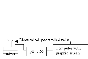
For acid-base titration, a modern lab will usually monitor titration with a pH meter which is interfaced to a computer, so that you will be able to plot the pH or other physical quantities versus the volume that is added.

In this module, we simulate this experiment graphically without using chemicals. A program that simulates titrations of strong acids and strong bases is very easy, because the calculation of pH in this experiment is very simple.
An example of titration is the acetic acid and NaOH - strong base and weak acid - titration following the equation below.
\[\ce{HC2H4O2(aq)+OH^{-}(aq) → C2H4O2(aq)+H2O(l) }\]

Titration Curve
The plot of pH as a function of titrant added is called a titration curve. Let us take a look at a titration process:
Evaluate \(\ce{[H+]}\) and pH in the titration of 10.0 mL 1.0 M \(\ce{HCl}\) solution with 1.0 M \(\ce{NaOH}\) solution, and plot the titration curve.
Solution
\(\begin{align}
\textrm{The amount of acid present} &= \mathrm{V_a\times C_a}\\
&= \mathrm{10.0\: mL \times \dfrac{1.0\: mol}{1000\: mL}}\\
&= \textrm{10 mmol (mili-mole)}
\end{align}\)
\(\textrm{The amount of base NaOH added} = \mathrm{V_b\times C_b}\)
\(\textrm{The amount of acid left} = \mathrm{V_a\times C_a - V_b\times C_b}\)
\(\textrm{The concentration of acid and thus }\ce{[H+]}
= \mathrm{\dfrac{[V_a\times C_a - V_b\times C_b]}{V_a + V_b}}\)
With the above formulation, we can build a table for various values as shown on the right.
| Base added | \(\ce{[H+]}\) | pH |
|---|---|---|
| 0 | 1.0 | 0.0 |
| 1.0 | 9/11 | 0.087 |
| 2.0 | 8/12 | 0.176 |
| 5.0 | 5/15 | 0.477 |
| Half- equivalence point | ||
| 8.0 | 2/18 | 0.954 |
| 9.0 | 1/19 | 1.279 |
| 9.3 | 0.7/19.3 | 1.440 |
| 9.5 | 0.5/19.5 | 1.591 |
| 9.7 | 0.3/19.7 | 1.817 |
| 9.8 | 0.2/19.8 | 2.0 |
| 9.9 | 0.1/19.9 | 2.300 |
| 9.95 | 0.05/19.95 | 2.60 |
| 10 | \(\ce{H2O\rightleftharpoons H+ + OH-}\) pH = 7 \(\ce{NaCl}\) neutral salt |
|
| Base added | \(\ce{[OH- ]}\) | pH |
| 10.05 | 0.05/20.05 | 11.397 |
| 10.10 | 0.5/20.1 | 11.697 |
| 11.0 | 1/21 | 12.678 |
| 15.0 | 5/25 | 13.301 |
| 20.0 | 20/30 | 13.924 |
Working to learn
Plot the titration curve on a graph based on the data.
Answer the following questions.
At equivalence point, why is pH=7? What formula is used to calculate pH?
Why does pH change rapidly at the equivalence point?
Sketch titration curves when the concentrations of both acids and bases are 0.10, 0.0010 and 0.000010 M. What can you conclude from these sketches?
What are \(\ce{[Na+]}\) and \(\ce{[Cl- ]}\) at the following points: initially (before any base is added), half-equivalence point; equivalence point, after 10.5 mL \(\ce{NaOH}\) is added, after 20.0 mL \(\ce{NaOH}\) is added?
Well, when you have acquired the skill to calculate the pH at any point during titration, you may write a simulation program to plot the titration curve. Calculations for strong-acid_strong-base titration are simple, but when weak acid or base are involved, the calculations are somewhat more complicated. However, we are interested in this area and some simulation programs are available on the internet.
Questions
- What are the pH of solutions of 10, 1.0, 0.10, 0.010 and 0.0010 M \(\ce{HCl}\)?
- What are \(\ce{[H+]}\) and the pH at the half equivalence point when a solution of 1.0 M \(\ce{HCl}\) is titrated by a 1.0 \(\ce{NaOH}\) solution?
- What are \(\ce{[Na+]}\) at the half equivalence point when a solution of 1.0 M \(\ce{HCl}\) is titrated by a 1.0 \(\ce{NaOH}\) solution?
- What are \(\ce{[H+]}\) and the pH at the equivalence point when a solution of 1.0 M \(\ce{HCl}\) is titrated by a 1.0 \(\ce{NaOH}\) solution?
- What are \(\ce{[Na+]}\) and \(\ce{[Cl- ]}\) at the equivalence point when a solution of 1.0 M \(\ce{HCl}\) is titrated by a 1.0 \(\ce{NaOH}\) solution?
- What are \(\ce{[H+]}\) and the pH of 1.0 M acetic acid solution? Ka = 1.8e-5
- What is the pH of the above solution when half of the acid is neutralized by \(\ce{NaOH}\) in the titration?
- What is the pH of the end point or equivalence point when 1.0 M acetic acid is titrated by 1.0 M \(\ce{NaOH}\) solution?
- A 0.10 M acetic acid solution is titrated with a 0.10 M \(\ce{NaOH}\) solution to the equivalence point. What is the concentration of the acetate ion?
Solutions
- Answer pH = -1, 0, 1, 2, and 3
Consider...
No calculators should be used. - Answer \(\mathrm{[H^+] = 0.333}\); pH = 0.477
Consider...
Do not forget the dilution factor. - Answer \(\mathrm{[H^+] = 0.333}\);
Consider...
What about \(\ce{[Cl- ]}\)? - Answer \(\ce{[H+]} = \textrm{1e-7}\); pH = 7
Consider...
This is only a theoretical value. - Answer \(\ce{[Ca+]} = \ce{[Cl- ]} = 0.5\)
Consider...
Note that \(\ce{[H+]}\) is balanced by \(\ce{[OH- ]}\), amd \(\ce{[Na+]}\) is balanced by \(\ce{[Cl- ]}\).
Most students usually forget the salt resulting from the titration. - Answer \(\ce{[H+]}=0.00424\); pH = 2.37
Consider...
The approximation \(\ce{[H+]}=(C K_{\ce a})^{1/2}\) can be used. - Answer pH = 4.74
Consider...
Do you know why pH = pKa in this case? At this point, the solution is a very good buffer. - Answer \(\ce{[OH- ]}=1.18\textrm{e-}4\); pOH = 4.78; pH = 9.22
Consider...
Justify the following formula for this condition. \(\ce{[OH- ]}=(K_{\ce w}/K_{\ce a}\times C)^{1/2}\)What is the pH of a 0.5 M sodium acetate solution?
- Answer 0.05 M
Consider...
You have doubled the volume in this case, and the concentration is 0.05 M sodium acetate.

