5.1: Carnot Cycle

The main contribution of Carnot to thermodynamics is his abstraction of the steam engine’s essential features into a more general and idealized heat engine. The definition of Carnot’s idealized cycle is as follows:

Definition: Carnot Cycle

A Carnot cycle is an idealized process composed of two isothermal and two adiabatic transformations. Each transformation is either an expansion or a compression of an ideal gas. All transformations are assumed to be reversible, and no energy is lost to mechanical friction.

A Carnot cycle connects two “heat reservoirs” at temperatures \(T_h\) (hot) and \(T_l\) (low), respectively. The reservoirs have a large thermal capacity so that their temperatures are unaffected by the cycle. The system is composed exclusively by the ideal gas, which is the only substance that changes temperature throughout the cycle. If we report the four transformations of a Carnot cycle on a \(PV\) diagram, we obtain the following plot:

Figure \(\PageIndex{1}\): PV-Diagram of a Carnot Cycle.

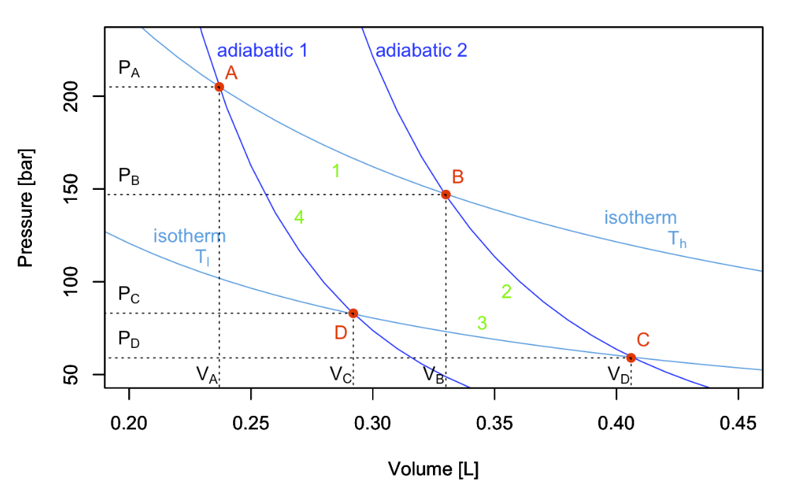
Stage 1: isothermal expansion \(A \rightarrow B\)

At this stage heat is released from the hot reservoir and is absorbed by the ideal gas particles within the system. Thus, the temperature of the system rises. The high temperature causes the gas particles to expand; pushing the piston upwards and doing work on the surroundings.

Figure \(\PageIndex{2}\)

Starting the analysis of the cycle from point \(A\) in Figure \(\PageIndex{1}\),\(^1\) the first transformation we encounter is an isothermal expansion at \(T_h\). Since the transformation is isothermal:

\[ \Delta U_1 = \overbrace{W_1}^{<0} + \overbrace{Q_1}^{>0} = 0 \Rightarrow Q_1 = -W_1, \nonumber \]

and heat and work can be calculated for this stage using Equation 2.4.14:

\[\begin{equation} \begin{aligned} Q_1 & = \left| Q_h \right| = nRT_h \overbrace{\ln \dfrac{V_B}{V_A}}^{>0 \text{ since } V_B>V_A} > 0, \\ W_1 & = -Q_1 = - nRT_h \ln \dfrac{V_B}{V_A} < 0, \end{aligned} \end{equation} \nonumber \]

where we denoted \(\left| Q_h \right|\) the absolute value of the heat that gets into the system from the hot reservoir.

Stage 2: adiabatic expansion \(B \rightarrow C\)

At this stage expansion continues, however there is no heat exchange between system and surroundings. Thus, the system is undergoing adiabatic expansion. The expansion allows the ideal gas particles to cool, decreasing the temperature of the system.

Figure \(\PageIndex{3}\)

The second transformation is an adiabatic expansion between \(T_h\) and \(T_l\). Since we are at adiabatic conditions:

\[ Q_2 = 0 \Rightarrow \Delta U_2 = W_2, \nonumber \]

and the negative energy (expansion work) can be calculated using:

\[ \Delta U_2 = W_2 = n \underbrace{\int_{T_h}^{T_l} C_V dT}_{<0 \text{ since } T_\mathrm{l}<T_\mathrm{h}} < 0. \nonumber \]

Stage 3: isothermal compression \(C \rightarrow D\)

At this stage the surroundings do work on the system which causes heat to be released (qc). The temperature within the system remains the same. Thus, isothermal compression occurs.

Figure \(\PageIndex{4}\)

The third transformation is an isothermal compression at \(T_l\). The formulas are the same as those used for stage 1, but they will results in heat and work with reversed signs (since this is a compression):

\[ \Delta U_3 = \overbrace{W_3}^{>0} + \overbrace{Q_3}^{<0} = 0 \Rightarrow Q_3 = -W_3, \nonumber \]

and:

\[\begin{equation} \begin{aligned} Q_3 & = \left| Q_l \right| = nRT_l \overbrace{\ln \dfrac{V_D}{V_C}}^{<0 \text{ since } V_D<V_C} < 0 , \\ W_3 & = -Q_3 = - nRT_l \ln \dfrac{V_D}{V_C} > 0, \end{aligned} \end{equation} \nonumber \]

where \(\left| Q_l \right|\) is the absolute value of the heat that gets out of the system to the cold reservoir (\(\left| Q_l \right|\) being the heat entering the system).

Stage 4: adiabatic compression \(D \rightarrow A\)

No heat exchange occurs at this stage, however, the surroundings continue to do work on the system. Adiabatic compression occurs which raises the temperature of the system as well as the location of the piston back to its original state (prior to stage one).

Figure \(\PageIndex{5}\)

The fourth and final transformation is an adiabatic comprssion that restores the system to point \(A\), bringing it from \(T_l\) to \(T_h\). Similarly to stage 3:

\[ Q_4 = 0 \Rightarrow \Delta U_4 = W_4, \nonumber \]

Since we are at adiabatic conditions. The energy associated with this process is now positive (compression work), and can be calculated using:

\[ \Delta U_4 = W_4 = n \underbrace{\int_{T_l}^{T_h} C_V dT}_{>0 \text{ since } T_\mathrm{h}>T_\mathrm{l}} > 0. \nonumber \]

Notice how \(\Delta U_4 = - \Delta U_2\) because \(\int_x^y=-\int_y^x\).

---

1. ︎The stages of a Carnot depicted at the beginning of each of this section and the following three ones are genetaken from Wikipedia, and have been generated and distributed by Author BlyumJ under CC-BY-SA license.︎