2.4: Calculation of Work

In thermodynamics, work (\(W\)) is the ability of a system to transfer energy by exerting a force on its surroundings. Work can be measured simply by evaluating its effects, such as displacing a massive object by some amount of space. The mathematical treatment of work, however, is complicated because work is a path function. In the following sections, we will analyze how work is calculated in some prototypical situations commonly encountered in the thermodynamical treatment of systems.

Figure \(\PageIndex{1}\): Isothermal Expansion of an Ideal Gas Against a Constant External Pressure.

Let’s consider the situation in Figure \(\PageIndex{1}\), where a special beaker with a piston that is free to move is filled with an ideal gas. The beaker sits on a desk, so the piston is not subject to any external forces other than the external pressure, \(P_{\text{ext}}\), and the internal pressure of the gas, \(P\). ¹ The piston is initially compressed to a position that is not in equilibrium \((i)\). After the process, the piston reaches a final equilibrium position \((f)\). How do we calculate the work (\(W\)) performed by the system?

From basic physics, we recall that the infinitesimal amount of work associated with an object moving in space is given by the force acting on the object (\(F\)) multiplied by the infinitesimal amount it gets displaced (\(d h\)):

\[ đ W = - Fdh, \label{2.4.1} \]

where the negative sign comes from the chemistry sign convention, Definition: System-centric, since the work in Figure \(\PageIndex{1}\) is performed by the system (expansion). What kind of force is moving the piston? It is the force due to the pressure of the gas. Relying upon another definition from physics, the pressure is the ratio between the force (\(F\)) and the area (\(A\)) that such force acts upon:

\[ P = F/A. \label{2.4.2} \]

Obtaining \(F\) from Equation \ref{2.4.2} and replacing it in Equation \ref{2.4.1}, we obtain:

\[ đ W - P \underbrace{Adh}_{dV}, \label{2.4.3} \]

and considering that \(Adh\) (area times infinitesimal height) is the definition of an infinitesimal volume \(dV\), we obtain:

\[ đ W = - PdV, \label{2.4.4} \]

If we want to calculate the amount of work performed by a system, \(W\), from Equation \ref{2.4.4}, we need to recall that \(đ W\) is an inexact differential. As such, we cannot integrate it from initial to final as for the (exact) differential of a state function, because:

\[ \int_{i}^{f}đ W \neq W_f - W_i, \label{2.4.5} \]

but rather:

\[ \int_{\text{path}} đ W = W, \label{2.4.6} \]

where the integration is performed along the path. Using Equation \ref{2.4.6}, we can integrate Equation \ref{2.4.4} as:

\[ \int đ W = W = - \int_{i}^{f} PdV, \label{2.4.7} \]

where the integral on the left-hand side is taken along the path,² while the integral on the right-hand side can be taken between the initial and final states, since \(dV\) is a state function. How do we solve the integral in Equation \ref{2.4.7}? It turns out that there are many different ways to solve this integral (perhaps not surprisingly, since the left-hand side depends on the path), which we will explore in the next section.

\(| W_{\text{max}} |\) and \(| W_{\text{min}} |\) in processes at constant temperature (isothermal)

At constant temperature, the piston in Figure \(\PageIndex{1}\) moves along the following PV diagram (this curve is obtained from an ideal gas at constant \(T=298\) K):

An expansion of the gas will happen between \(P_i\) and \(P_f\). If the expansion happens in a one-step fast process, for example against external atmospheric pressure, then we can consider such final pressure constant (for example \(P_f=P_{\text{ext}} =1\;\mathrm{bar}\)), and solve the integral as:

\[ W_{\text{1-step}} = - \int_{i}^{f} P_{\text{ext}}dV = -P_{\text{ext}} \int_{i}^{f} dV = -P_{\text{ext}} (V_f-V_i), \label{2.4.8} \]

Notice how the work is negative, since during an expansion the work is performed by the system (recall the chemistry sign convention). The absolute value of the work³ represents the red area of the PV-diagram:

\[ \left| W_{\text{1-step}} \right| = P_{\text{ext}} (V_f-V_i) \label{2.4.9} \]

If the process happens in two steps by pausing at an intermediate position (1) until equilibrium is reached, then we should calculate the work by dividing it into two separate processes, \(A\) and \(B\), and solve each one as we did in the previous case. The first process is an expansion between \(P_i\) and \(P_1\), with \(P_1\) constant. The absolute value of the work, \(W_A\), is represented by the blue area:

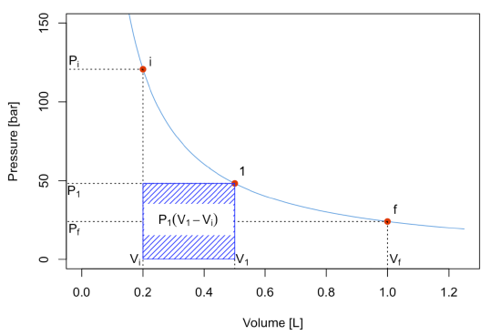
\[ \left| W_A \right| = P_1 (V_1-V_i) \label{2.4.10} \]

The second process is an expansion between \(P_1\) and \(P_f\), with \(P_f=P_{\text{ext}}\) constant. The absolute value of the work for this second process is represented by the green area:

\[ \left| W_B \right| = P_f (V_f-V_1) \label{2.4.11} \]

The total absolute value of the work for the 2-step process is given by the sum of the two areas:

\[ \left| W_{\text{2-step}} \right| = \left| W_A \right| + \left| W_B \right| = P_1 (V_1-V_i)+P_f (V_f-V_1). \label{2.4.12} \]

As can be easily verified by comparing the shaded areas in the plots, \(\left| W_{\text{2-step}} \right| > \left| W_{\text{1-step}} \right|\).

We can easily extend this procedure to consider processes that happens in 3, 4, 5, …, \(n\) steps. What is the limit of this procedure? In other words, what happens when \(n \rightarrow \infty\)? A simple answer is given by the plots in the next Figure, which clearly demonstrates that the maximum value of the area underneath the curve \(\left| W_{\text{max}}\right|\) is achieved in an \(\infty\)-step process, for which the work is calculated as:

\[ \left| W_{\infty \text{-step}} \right| = \left| W_{\text{max}} \right| = \sum_{n}^{\infty} P_n(V_n-V_{n-1}) = \int_{i}^{f} PdV. \label{2.4.13} \]

The integral on the right hand side of Equation \ref{2.4.13} can be solved for an ideal gas by calculating the pressure using the ideal gas law \(P=\dfrac{nRT}{V}\), and solving the integral since \(n\), \(R\), and \(T\) are constant:

\[ \left| W_{\text{max}} \right| = nRT \int_{i}^{f} \dfrac{dV}{V} = nRT \ln \dfrac{V_f}{V_i}. \label{2.4.14} \]

This example demonstrates why work is a path function. If we perform a fast 1-step expansion, the system will perform an amount of work that is much smaller than the amount of work it can perform if the expansion between the same points happens slowly in an \(\infty\)-step process.

The same considerations that we made up to this point for expansion processes hold specularly for compression ones. The only difference is that the work associated with compressions will have a positive sign since it must be performed onto the system. As such, the amount of work for a transformation that happens in a finite amount of steps will be an upper bound to the minimum amount of work required to compress the system.⁴ \(\left| W_{\text{min}} \right|\) for compressions is calculated as the area underneath the PV curve, exactly as \(\left| W_{\text{min}} \right|\) for expansions in Equation \ref{2.4.13}.

---

1. For this simple thought experiment, we will ignore any external force that is not significant. In other words, we will not consider the friction of the piston on the beaker walls or any other foreign influence.︎
2. from here on we will replace the notation \(\int_{\text{path}}\) with the more convenient \(\int\) and we will keep in mind that the integral of an inexact differential must be taken along the path.︎
3. we use the absolute value to avoid confusions due to the fact that the expansion work is negative according to Definition: System-centric.︎
4. In contrast to a lower bound for expansion processes.