Solid State NMR Experimental Setup

Performing a MAS Experiment

This section is devoted to giving a practical guide for solid state NMR. Please follow all safety guidelines at your University. All experiments are performed on a 500MHz magnet using a Bruker AQS spectrometer running TopSpin 2.1. Please note that your spectrometer may be different and/or run different software in which some/all of the commands listed below will be different.

The Probe

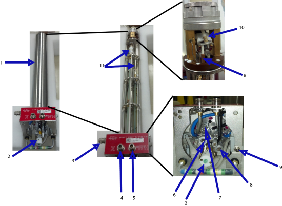
The probe has several different parts which are summarized below. The probe must house the sample, spin the sample, tune to the correct frequency, and allow for temperature dependence studies. 

1. Probe Casing: The probe case shields the delicate components inside the probe. It is typically made out of aluminum and attaches to the base of the probe via a series of screws.
2. Variable Temperature (VT) line and Bearing Airline: The VT line is a glass rod that connects to the VT apparatus coming out the the liquid nitrogen dewar (see section x.x). It transfers the cold nitrogen gas to the sample 
3. Drive Airline
4. X Channel
5. ¹H Channel
6. X Channel Tuning Rod
7. X Channel Matching Rod
8. Magic Angle Adjustment Rod
9. Tachometer
10. Stator (Coil contained inside)
11. Variable capacitors for matching and tuning

Packing The Sample

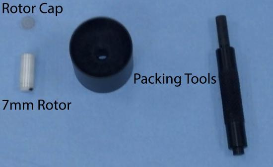
It becomes very important in SSNMR to pack your sample very carefully. The sample is rotating several thousands of times per second and therefore must not wobble or suddenly stop. If the sample stops rotating in the stador, it will crash and this normally breaks the stater results in a several thousand dollar repair. In order to prevent this here are some steps to pack the sample.

1. Crush the sample thoroughly. Use an mortar and pestle. crush your sample into a fine powder by constantly grinding the sample for about 10 minutes. Not only does this help with the packing efficiency allowing for more sample to be added, but it also homogenizes the crystallite orientations. 
2. Place the rotor in the packing tool. 
3. Add a small amount of sample to the rotor. Next, using the packing stick, press the sample down into the bottom of the rotor. I normally make about 10-15 quick downward pushes to allow the sample to find its closest packing arrangement, then I press it hard into the bottom using the tool about 5 times.
4. Repeat Step 3 until the rotor is almost full
5. When your about to the top, you need to leave a little room to put in the cap. This is primarily the part when people tend to mess up packing. There can be no loose powder at the top. Therefore you must carefully push on the cap without shaking any loose powder at the top. If you're not interested in 13C or 1H NMR placing some Parafilm on top of the sample can prevent this from happening. 
6. Place the cap on the rotor. Be careful not to put it on at an angle and the it fully closes. If there is a space between the rotor and the cap, you have too much sample and you need to unpack some of it. 
7. Mark the bottom of the rotor with a black sharpie so the tachometer can read the spinning speed.

Spinning The Sample

To spin the sample, you must first insert the sample into the stador. Most probes are equipped with transfer lines that use compressed air to insert and eject samples. Once the sample is inserted, you may begin spinning the sample. Most spectrometers have a automatic program that will allow you to spin the sample by simply selecting the spinning speed you want. However, you may need to do it manually, wither on the console or by opening the air valves. When doing this it is important to have the bearing air at least 150 mbar higher than the drive pressue. This keeps the sample elevated and from crashing into the sides of the rotor. When stopping the rotor, you must slowly decrease the spinning speed or else you risk crashing the rotor.

Setting Up The Spectrometer

Once the sample is spinning, it is now important to make sure all of the hardware is set. The first thing to do is select the probe that you are using by typing "edhead" this brings up a list of available probes. Select the one you have already inseted your sample into. After selecting this, the screen will show the current hardware set up, along with the nucleus you will be probing. If this is not correct, select the nucleus you are interested in. You will also be able to see the frequency at which this nucleus is resonant at. 

Next, make sure the band pass filter is selected for the RF range you are interested in. If you do not have the correct filter, then all the signal will be locked and your experiment will not collect any data. 

Next read in the shim file. The shims are used to homogenize the field. type rsh to read in the shim profile for your probe.

Tuning The Probe

The probe must be tuned to the correct frequency range in order to probe the transitions. Additionally, the RF circuit must match impedance with the spectrometer, which is known as matching. To tune the probe here are the steps:

1. Type "wobb" on the command line.
2. Rotate the tuning rod clockwise if the tuning line needs increase in frequency and counter clockwise to decrease the frequency. 
3. Use the matching rod to lower the line as low as it goes.
4. Once optimized, type "stop"

Note: you may need to increase sweep width on the wobble curve to see the line. You may change this under acquisition parameters.

Running the Experiment

Running the experiment is actually fairly easy, however there are several parameters which need to be addressed.

• Experiment: You can choose which experiment to run. Press the "..." next to the spectrometer and select "zg" for a simple pulse and acquire experiment.
• TD: This is the number of points your FID will consist of. Each data point will be acquired after a delay of DW
• NS: The is the number of scans which is to be completed for the experiment. It must be an integer number of the phase cycle. For MAS this is 8.
• SW: This is the sweep width in Hz of your spectrum. This must be large enough for your experimental spectrum to be seen. It is equal to 1/DW
• AQ: This is the acquisition time which is automatically set by TD*DW. Typically 1ms is long enough 
• DW: The is the dwell time. The dwell time is the amount of time waited between individual points being sampled. A typical value for this is 5us.
• DS: This is the dummy scans which the experiment is performed but no data is acquired. The dummy scans are first completed then NS scans are completed.
• RG: This is the receiver gain. The receiver gain amplifies the signal. This is sample dependent. If the FID looks clipped i.e. looks like the tops of the peaks are being cut off in the time dimension, then the RG needs to be lowered.
• P1: This is the pulse length. You can calibrate this using "popt" command. The popt command will bring you to a separate window in which you define the parameter you would like to optimize. Type p1. Next, type in the minimum pulse length you want to sample and the interval you want to increment with. Press start and the maximum peak is the 90 degree pulse. 
• PL1: The power level at which the pulse, P1, is delivered. This is in decibels so smaller numbers are high power.
• SFO1: This is the carrier frequency which is set by the nucleus of interest.
• D1: This is the amount of tiume between each scan. It should be approximately 5*T1 for good spectra to be acquired.

After there parameters are set, type "zg" to begin the experiment. It will complete NS scans and the time to complete it will be approximately NS*D1.

Running Variable Temperature Experiments

Exporting Data and Bruker Output files