Hyperfine Structure
- Page ID
- 96679
\( \newcommand{\vecs}[1]{\overset { \scriptstyle \rightharpoonup} {\mathbf{#1}} } \)
\( \newcommand{\vecd}[1]{\overset{-\!-\!\rightharpoonup}{\vphantom{a}\smash {#1}}} \)
\( \newcommand{\dsum}{\displaystyle\sum\limits} \)
\( \newcommand{\dint}{\displaystyle\int\limits} \)
\( \newcommand{\dlim}{\displaystyle\lim\limits} \)
\( \newcommand{\id}{\mathrm{id}}\) \( \newcommand{\Span}{\mathrm{span}}\)
( \newcommand{\kernel}{\mathrm{null}\,}\) \( \newcommand{\range}{\mathrm{range}\,}\)
\( \newcommand{\RealPart}{\mathrm{Re}}\) \( \newcommand{\ImaginaryPart}{\mathrm{Im}}\)
\( \newcommand{\Argument}{\mathrm{Arg}}\) \( \newcommand{\norm}[1]{\| #1 \|}\)
\( \newcommand{\inner}[2]{\langle #1, #2 \rangle}\)
\( \newcommand{\Span}{\mathrm{span}}\)
\( \newcommand{\id}{\mathrm{id}}\)
\( \newcommand{\Span}{\mathrm{span}}\)
\( \newcommand{\kernel}{\mathrm{null}\,}\)
\( \newcommand{\range}{\mathrm{range}\,}\)
\( \newcommand{\RealPart}{\mathrm{Re}}\)
\( \newcommand{\ImaginaryPart}{\mathrm{Im}}\)
\( \newcommand{\Argument}{\mathrm{Arg}}\)
\( \newcommand{\norm}[1]{\| #1 \|}\)
\( \newcommand{\inner}[2]{\langle #1, #2 \rangle}\)
\( \newcommand{\Span}{\mathrm{span}}\) \( \newcommand{\AA}{\unicode[.8,0]{x212B}}\)
\( \newcommand{\vectorA}[1]{\vec{#1}} % arrow\)
\( \newcommand{\vectorAt}[1]{\vec{\text{#1}}} % arrow\)
\( \newcommand{\vectorB}[1]{\overset { \scriptstyle \rightharpoonup} {\mathbf{#1}} } \)
\( \newcommand{\vectorC}[1]{\textbf{#1}} \)
\( \newcommand{\vectorD}[1]{\overrightarrow{#1}} \)
\( \newcommand{\vectorDt}[1]{\overrightarrow{\text{#1}}} \)
\( \newcommand{\vectE}[1]{\overset{-\!-\!\rightharpoonup}{\vphantom{a}\smash{\mathbf {#1}}}} \)
\( \newcommand{\vecs}[1]{\overset { \scriptstyle \rightharpoonup} {\mathbf{#1}} } \)
\(\newcommand{\longvect}{\overrightarrow}\)
\( \newcommand{\vecd}[1]{\overset{-\!-\!\rightharpoonup}{\vphantom{a}\smash {#1}}} \)
\(\newcommand{\avec}{\mathbf a}\) \(\newcommand{\bvec}{\mathbf b}\) \(\newcommand{\cvec}{\mathbf c}\) \(\newcommand{\dvec}{\mathbf d}\) \(\newcommand{\dtil}{\widetilde{\mathbf d}}\) \(\newcommand{\evec}{\mathbf e}\) \(\newcommand{\fvec}{\mathbf f}\) \(\newcommand{\nvec}{\mathbf n}\) \(\newcommand{\pvec}{\mathbf p}\) \(\newcommand{\qvec}{\mathbf q}\) \(\newcommand{\svec}{\mathbf s}\) \(\newcommand{\tvec}{\mathbf t}\) \(\newcommand{\uvec}{\mathbf u}\) \(\newcommand{\vvec}{\mathbf v}\) \(\newcommand{\wvec}{\mathbf w}\) \(\newcommand{\xvec}{\mathbf x}\) \(\newcommand{\yvec}{\mathbf y}\) \(\newcommand{\zvec}{\mathbf z}\) \(\newcommand{\rvec}{\mathbf r}\) \(\newcommand{\mvec}{\mathbf m}\) \(\newcommand{\zerovec}{\mathbf 0}\) \(\newcommand{\onevec}{\mathbf 1}\) \(\newcommand{\real}{\mathbb R}\) \(\newcommand{\twovec}[2]{\left[\begin{array}{r}#1 \\ #2 \end{array}\right]}\) \(\newcommand{\ctwovec}[2]{\left[\begin{array}{c}#1 \\ #2 \end{array}\right]}\) \(\newcommand{\threevec}[3]{\left[\begin{array}{r}#1 \\ #2 \\ #3 \end{array}\right]}\) \(\newcommand{\cthreevec}[3]{\left[\begin{array}{c}#1 \\ #2 \\ #3 \end{array}\right]}\) \(\newcommand{\fourvec}[4]{\left[\begin{array}{r}#1 \\ #2 \\ #3 \\ #4 \end{array}\right]}\) \(\newcommand{\cfourvec}[4]{\left[\begin{array}{c}#1 \\ #2 \\ #3 \\ #4 \end{array}\right]}\) \(\newcommand{\fivevec}[5]{\left[\begin{array}{r}#1 \\ #2 \\ #3 \\ #4 \\ #5 \\ \end{array}\right]}\) \(\newcommand{\cfivevec}[5]{\left[\begin{array}{c}#1 \\ #2 \\ #3 \\ #4 \\ #5 \\ \end{array}\right]}\) \(\newcommand{\mattwo}[4]{\left[\begin{array}{rr}#1 \amp #2 \\ #3 \amp #4 \\ \end{array}\right]}\) \(\newcommand{\laspan}[1]{\text{Span}\{#1\}}\) \(\newcommand{\bcal}{\cal B}\) \(\newcommand{\ccal}{\cal C}\) \(\newcommand{\scal}{\cal S}\) \(\newcommand{\wcal}{\cal W}\) \(\newcommand{\ecal}{\cal E}\) \(\newcommand{\coords}[2]{\left\{#1\right\}_{#2}}\) \(\newcommand{\gray}[1]{\color{gray}{#1}}\) \(\newcommand{\lgray}[1]{\color{lightgray}{#1}}\) \(\newcommand{\rank}{\operatorname{rank}}\) \(\newcommand{\row}{\text{Row}}\) \(\newcommand{\col}{\text{Col}}\) \(\renewcommand{\row}{\text{Row}}\) \(\newcommand{\nul}{\text{Nul}}\) \(\newcommand{\var}{\text{Var}}\) \(\newcommand{\corr}{\text{corr}}\) \(\newcommand{\len}[1]{\left|#1\right|}\) \(\newcommand{\bbar}{\overline{\bvec}}\) \(\newcommand{\bhat}{\widehat{\bvec}}\) \(\newcommand{\bperp}{\bvec^\perp}\) \(\newcommand{\xhat}{\widehat{\xvec}}\) \(\newcommand{\vhat}{\widehat{\vvec}}\) \(\newcommand{\uhat}{\widehat{\uvec}}\) \(\newcommand{\what}{\widehat{\wvec}}\) \(\newcommand{\Sighat}{\widehat{\Sigma}}\) \(\newcommand{\lt}{<}\) \(\newcommand{\gt}{>}\) \(\newcommand{\amp}{&}\) \(\definecolor{fillinmathshade}{gray}{0.9}\)Splittings from Internal Magnetic Field of Nuclear Spins
The hyperfine structure is caused by interaction between magnetic field (from electron movement) and nuclear spin. For instance, the hydrogen atom has one proton with spin \(I = ½\) and corresponding magnetic moment
\[ \vec{\mu}_P = −g_I \dfrac{eh}{2m_p} \dfrac{\vec{I}}{\hbar} = \dfrac{µ_K\vec{I}}{hbar} \]
Since a proton is heavier than an electron, its magneton \(µ_K\)
\[µ_K = g_I \dfrac{eh}{2m_p}\]
is lighter by a factor \(\dfrac{m_e}{m_p}\).
Similar to fine structure coupling, we must connect \(\vec{J}\) and \(\vec{I}\) now having "new" total angular momentum:
\[\vec{F} = \vec{J} + \vec{I}\]
where
\[\hat{F}^2 |\psi \rangle = F(F +1) h^ | \psi \rangle\]
and
\[ \hat{F}_z | \psi \rangle= m_F \hbar | \psi \rangle\]
where
\[m_F = −F, −F+1, ... , F−1, F\]
Squaring the equation for \(\vec{F}\) and solving it relatively \(\vec{J} \cdot \vec{I}\) one can obtain the hyperfine energy structure:
\[E_{HFS} = \dfrac{cHFS}{2}\{F(F + 1) - J(J + 1) - I(I + 1)\}\]
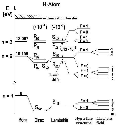
The lowest term of hydrogen 1²S½ is then split into two terms with F = 1 (spin electron and spin proton ) and F = 0 (spin electron and spin proton ¯ antiparallel). The transition between these two levels can only occur when the spin turns over. This, however, is a very rare phenomenon in an isolated hydrogen atom (it, on average, would happen once every 10 million years for a single molecule) however because of the exceedingly high number of hydrogen atoms in the universe it can be observed. Further, collisions can flip the spin. It lies near n» 1,4204 GHz (λ = 21 cm).
Photons have Angular Momenta Too
Since this transition changes the system angular momentum from \(F = 1h\) into \(F = 0h\) but from the fact that the total angular momentum should be the same follows photon must take the hydrogen atom angular momentum. And so a photon also possesses angular momentum. However, the photon spin is as follows
\[S_{Photon} = 1\,h\]
The photon spin isn't a good designation because the "photon spin" projection on the flight axis can take values m = +1 or m = -1 for right- and lefthand circular polarized light, correspondingly. And it can never be m=0, that would correspond to the longitudinal polarization which is never realized!
The proton spin has interesting consequences for optical spectra since we obtain the selection rule for transitions. We will have for the final total angular momentum \(\vec{J_f}\) of the system that was originally at some initial state \(\vec{J_i}\) according to the angular momentum conservation law:
\[ \vec{J}_i = \vec{J}_f + \vec{J}_{photon}\]
Certainly \(\vec{J}_{photon}\) shouldn't be necessarily equal to \(\vec{1}\) because photon can also possess (together with spin) the orbital moment relative to an atom. The photon emission with unchanged orbital moment visually means that photon has left the boundary areas. Nevertheless, this process is very improbable so that quantum numbers \(J_i\) and \(J_f\) have the following relation according to the angular momentum conservation law:
\[ΔJ = J_f − J_i = 0,\, ±1\]

- \[ΔJ = −1\]
- \[ΔM = 0 , ±1\]
P-Branch
- ΔJ = 0
- ΔM = ±1
Q-Branch
- ΔJ = +1
- ΔM = 0 , ±1
R-Branch
If \(J_f = 0\) and \(J_i = 0\) then \(ΔJ=0\) is forbidden according to the angular momentum conservation law. If there is small interaction between \(\vec{L}\) and \(\vec{S}\) then there is special selection rule for spin that states:
\[ΔS = 0\]

The selection rule for electron orbital moment has been given here without any derivation:
\[Δl = ±1\]
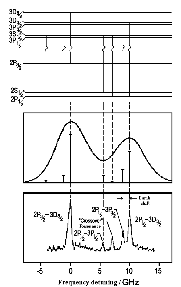
The possible transitions are shown on the illustration to the left (Balmer a-Line, n = 3 ↔ n = 2). Since H atoms move there are Doppler distribution of these optical lines, that can be resolved by using Doppler free spectroscopy which can help us to prove the theory.
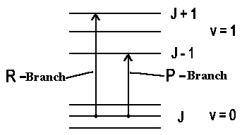
Certainly we must also have angular momentum conservation for increasing rotation of a molecule. In the simplest case of a linear molecule for which electron contribution into angular momentum is small so that \(ΔJ = ±1\), i.e. the rotation can be increased by \(1h\) or decreased by \(1h\) when photon is absorbed. It's said about P-Branch (the rotation is decreased by 1h) and R-Branch (the rotation is increased by 1h).
If total electron angular momentum is not equal to 0 or if we have a deal with a non-linear molecule then the kinetic impulse vector character according to the selection rule undergoes some changes, i.e. there is also a transition \(\Delta J = 0\) (Q-Branch) possible (when \(J = 0 → J = 0 !).

In Raman-Spectroscopy two photons are used: the molecule undergoes a transition from the initial state i into virtual state and then there is "emission" from this virtual state into the final state f. Since the angular momentum of both photons should compensate or add up to each other (the angular momentum conservation law) it follows the selection rules for the Raman spectroscopy: ΔJ = 0, ±2. When ΔJ = 0 the angular momentums of both photons compensate each other (¯); and when ΔJ = ±2 they are added to each other ( or ¯¯). One can talk about S-Branch (ΔJ = +2) and O-Branch (ΔJ = -2) in this case.

