Fine Structure

From classical electrodynamics, a rotating electrically charged body creates a magnetic dipole with magnetic poles of equal magnitude but opposite polarity. This analogy holds as an electron indeed behaves like a tiny bar magnet. In the classical model, the electron (Bohr atom model) is moving along a closed path. A revolving electron is equivalent to a current loop (Figure \(\PageIndex{1a}\)).

Figure \(\PageIndex{1}\): The rotating electron (really intrinsic spin) of the electron induces a different magnet. (CC BY-SA OpenStax).

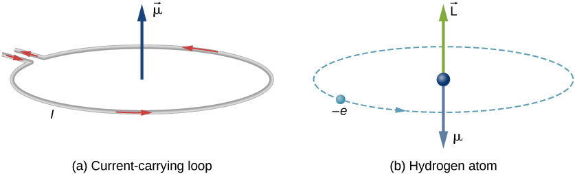
The current arising from the orbiting of the electron around the nucleus is

\[I = \dfrac{e}{T}\]

where \(T\) is the orbital period or revolution. We can define the velocity then as

\[v=\dfrac{2πr}{T} \]

where \(r\) is the radius of orbit. The "orbital" magnetic (dipole) moment is then

\[\vec{\mu}_L = \dfrac{\vec{\mu}e}{T} (π r^2) \label{eq1}\]

and the angular momentum associated with that orbital motion is

\[ \begin{align} L &= m_e v_r \\[4pt] &= \dfrac{m_e 2\pi r^2}{T} \label{eq2} \end{align}\]

and \(m_e\) is the electron rest mass.

Next we combine Equation \ref{eq1} and \ref{eq2} to get how the orbital angular momentum induced a magnetic moment (in vector form)

\[ \color{red} \vec{\mu}_L = - \dfrac{e}{2m_e} \vec{L} \label{classical}\]

For a more detailed derivation of Equation \ref{classical}, look here. We can glean two important feature from Equation \ref{classical}:

1. If the electron has zero orbital angular momentum, it will have a zero-amplitude orbital magnetic moment.
2. The orientation of the orbital angular moment is parallel to the angular momentum.

The Quantum Orbital Magnetic Dipole Moment

Equation \ref{classical} is applicable to classical systems and since \(\vec{L}\) can have any values (amplitude and orientation), so can the magnetic moment. That is a different story in the quantum world. where the orbital angular momentum is quantized and hence so is \(\mu_L\). The amplitude of is \(\vec{L}\) represented by the \(\hat{L}^2\) operator and the projection of \(\vec{L}\) on the z-axis is represented by \(\hat{L}_z\) operator.

\[\hat{L^2} | \psi \rangle = \ell(\ell+1) \hbar^2 | \psi \rangle\]

and

\[\hat{L}_z | \psi \rangle = m_l \hbar | \psi \rangle\]

So we obtain the eigenvalues \(µ_{L_z}\) of z-component of the magnetic moment

\[µ_{L_z} = −\dfrac{ e}{2m_e} \hbar m_l \label{eq5}\]

It is usual to express the magnetic moment (Equation \ref{eq5}) in terms the Bohr magneton \(\mu_B\)

\[µ_{L_z} = −µ_B \,m_l\]

where \(µ_B\) is the Bohr Magneton:

\[µ_B = \dfrac{e\hbar}{2m_e}\]

The Bohr magneton is a physical constant and the natural unit for expressing the magnetic moment of an electron caused by either its orbital angular momentum and (and spin as discussed below) and is numerically

\[\begin{align} µ_B &= 9.273 \times 10^{-24}\, J/K \\[4pt] &= 5.656 \times 10^{-5}\, eV/T \\[4pt] &= 1.4 \times 10^{10}\, Hz/T \,(T \,= \,Tesla) \end{align}\]

Coupling Orbital Magnetic Dipole Moment to an External Magnetic Field

When a magnetic field is applied to the electron, then the energies of the eigenstates will depends on the magnitude \(B\) of the applied magnetic field \(\vec{B}\) via

\[ \begin{align} E_B &= −µ_{L_z} \, B \\[4pt] &= µ_B\, m_l\, B \end{align}\]

and the total energy of that state is

\[\begin{align} E &= E_0 + E_B \\[4pt] &= E_0 + µ_B\, m_l\, B \end{align}\]

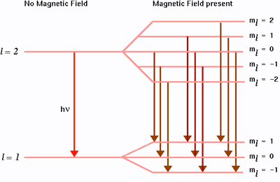
Hence, the energy levels having a angular momentum with quantum number \(\ell\) are split into \(2\ell + 1\) new levels (Figure \(\PageIndex{2}\)):

Figure \(\PageIndex{2}\): Splitting of spin-1/2 state into two in an external magnetic field

This effect is the "ordinary" or "normal" Zeeman Effect.

Figure \(\PageIndex{3}\): Splitting of single electron levels in an externally applied magnetic field.

Coupling Spin Magnetic Dipole Moment to an External Magnetic Field

The hydrogen ground state (\(m_l = 0\)) is uninfluenced in Figure \(\PageIndex{1}\). However, we know that a H atom is paramagnetic; this is because of electron spin. Now we consider the spin in classical mechanics as rotating around the axis electron. We also find here

\[µ_{S_z} = −g_S\, µ_B \, m_s \]

\[E_B = g_S\, µ_B\, m_s\, B\]

The so-called gyromagnetic factor \(g_S\) is obtained from the relativistic Dirac equation and experiments quantify it at

\[g_S = 2.00231930438(6)\]

The value

\[g_S\, µ_B ≈ 28\, GHz/T\]

shows us which energy state is higher according to electron spin interaction with magnetic field. Since now it's possible to produce magnetic fields with the strength of a few Teslas, we expect to detect transitions in GHz region (microwaves) when applying such fields. That's why Electron-Spin-Resonance (ESR) Spectroscopy is involved with microwaves. When applying NMR method we have a deal with MHz region. We will discuss it in more detail later.

Dec 2, 2017, 10:13 AM

http://www.pci.tu-bs.de/aggericke/Le...SR_NMR/NMR.htm