
WKB Approximation
- Page ID
- 66730
\( \newcommand{\vecs}[1]{\overset { \scriptstyle \rightharpoonup} {\mathbf{#1}} } \)
\( \newcommand{\vecd}[1]{\overset{-\!-\!\rightharpoonup}{\vphantom{a}\smash {#1}}} \)
\( \newcommand{\dsum}{\displaystyle\sum\limits} \)
\( \newcommand{\dint}{\displaystyle\int\limits} \)
\( \newcommand{\dlim}{\displaystyle\lim\limits} \)
\( \newcommand{\id}{\mathrm{id}}\) \( \newcommand{\Span}{\mathrm{span}}\)
( \newcommand{\kernel}{\mathrm{null}\,}\) \( \newcommand{\range}{\mathrm{range}\,}\)
\( \newcommand{\RealPart}{\mathrm{Re}}\) \( \newcommand{\ImaginaryPart}{\mathrm{Im}}\)
\( \newcommand{\Argument}{\mathrm{Arg}}\) \( \newcommand{\norm}[1]{\| #1 \|}\)
\( \newcommand{\inner}[2]{\langle #1, #2 \rangle}\)
\( \newcommand{\Span}{\mathrm{span}}\)
\( \newcommand{\id}{\mathrm{id}}\)
\( \newcommand{\Span}{\mathrm{span}}\)
\( \newcommand{\kernel}{\mathrm{null}\,}\)
\( \newcommand{\range}{\mathrm{range}\,}\)
\( \newcommand{\RealPart}{\mathrm{Re}}\)
\( \newcommand{\ImaginaryPart}{\mathrm{Im}}\)
\( \newcommand{\Argument}{\mathrm{Arg}}\)
\( \newcommand{\norm}[1]{\| #1 \|}\)
\( \newcommand{\inner}[2]{\langle #1, #2 \rangle}\)
\( \newcommand{\Span}{\mathrm{span}}\) \( \newcommand{\AA}{\unicode[.8,0]{x212B}}\)
\( \newcommand{\vectorA}[1]{\vec{#1}} % arrow\)
\( \newcommand{\vectorAt}[1]{\vec{\text{#1}}} % arrow\)
\( \newcommand{\vectorB}[1]{\overset { \scriptstyle \rightharpoonup} {\mathbf{#1}} } \)
\( \newcommand{\vectorC}[1]{\textbf{#1}} \)
\( \newcommand{\vectorD}[1]{\overrightarrow{#1}} \)
\( \newcommand{\vectorDt}[1]{\overrightarrow{\text{#1}}} \)
\( \newcommand{\vectE}[1]{\overset{-\!-\!\rightharpoonup}{\vphantom{a}\smash{\mathbf {#1}}}} \)
\( \newcommand{\vecs}[1]{\overset { \scriptstyle \rightharpoonup} {\mathbf{#1}} } \)
\(\newcommand{\longvect}{\overrightarrow}\)
\( \newcommand{\vecd}[1]{\overset{-\!-\!\rightharpoonup}{\vphantom{a}\smash {#1}}} \)
\(\newcommand{\avec}{\mathbf a}\) \(\newcommand{\bvec}{\mathbf b}\) \(\newcommand{\cvec}{\mathbf c}\) \(\newcommand{\dvec}{\mathbf d}\) \(\newcommand{\dtil}{\widetilde{\mathbf d}}\) \(\newcommand{\evec}{\mathbf e}\) \(\newcommand{\fvec}{\mathbf f}\) \(\newcommand{\nvec}{\mathbf n}\) \(\newcommand{\pvec}{\mathbf p}\) \(\newcommand{\qvec}{\mathbf q}\) \(\newcommand{\svec}{\mathbf s}\) \(\newcommand{\tvec}{\mathbf t}\) \(\newcommand{\uvec}{\mathbf u}\) \(\newcommand{\vvec}{\mathbf v}\) \(\newcommand{\wvec}{\mathbf w}\) \(\newcommand{\xvec}{\mathbf x}\) \(\newcommand{\yvec}{\mathbf y}\) \(\newcommand{\zvec}{\mathbf z}\) \(\newcommand{\rvec}{\mathbf r}\) \(\newcommand{\mvec}{\mathbf m}\) \(\newcommand{\zerovec}{\mathbf 0}\) \(\newcommand{\onevec}{\mathbf 1}\) \(\newcommand{\real}{\mathbb R}\) \(\newcommand{\twovec}[2]{\left[\begin{array}{r}#1 \\ #2 \end{array}\right]}\) \(\newcommand{\ctwovec}[2]{\left[\begin{array}{c}#1 \\ #2 \end{array}\right]}\) \(\newcommand{\threevec}[3]{\left[\begin{array}{r}#1 \\ #2 \\ #3 \end{array}\right]}\) \(\newcommand{\cthreevec}[3]{\left[\begin{array}{c}#1 \\ #2 \\ #3 \end{array}\right]}\) \(\newcommand{\fourvec}[4]{\left[\begin{array}{r}#1 \\ #2 \\ #3 \\ #4 \end{array}\right]}\) \(\newcommand{\cfourvec}[4]{\left[\begin{array}{c}#1 \\ #2 \\ #3 \\ #4 \end{array}\right]}\) \(\newcommand{\fivevec}[5]{\left[\begin{array}{r}#1 \\ #2 \\ #3 \\ #4 \\ #5 \\ \end{array}\right]}\) \(\newcommand{\cfivevec}[5]{\left[\begin{array}{c}#1 \\ #2 \\ #3 \\ #4 \\ #5 \\ \end{array}\right]}\) \(\newcommand{\mattwo}[4]{\left[\begin{array}{rr}#1 \amp #2 \\ #3 \amp #4 \\ \end{array}\right]}\) \(\newcommand{\laspan}[1]{\text{Span}\{#1\}}\) \(\newcommand{\bcal}{\cal B}\) \(\newcommand{\ccal}{\cal C}\) \(\newcommand{\scal}{\cal S}\) \(\newcommand{\wcal}{\cal W}\) \(\newcommand{\ecal}{\cal E}\) \(\newcommand{\coords}[2]{\left\{#1\right\}_{#2}}\) \(\newcommand{\gray}[1]{\color{gray}{#1}}\) \(\newcommand{\lgray}[1]{\color{lightgray}{#1}}\) \(\newcommand{\rank}{\operatorname{rank}}\) \(\newcommand{\row}{\text{Row}}\) \(\newcommand{\col}{\text{Col}}\) \(\renewcommand{\row}{\text{Row}}\) \(\newcommand{\nul}{\text{Nul}}\) \(\newcommand{\var}{\text{Var}}\) \(\newcommand{\corr}{\text{corr}}\) \(\newcommand{\len}[1]{\left|#1\right|}\) \(\newcommand{\bbar}{\overline{\bvec}}\) \(\newcommand{\bhat}{\widehat{\bvec}}\) \(\newcommand{\bperp}{\bvec^\perp}\) \(\newcommand{\xhat}{\widehat{\xvec}}\) \(\newcommand{\vhat}{\widehat{\vvec}}\) \(\newcommand{\uhat}{\widehat{\uvec}}\) \(\newcommand{\what}{\widehat{\wvec}}\) \(\newcommand{\Sighat}{\widehat{\Sigma}}\) \(\newcommand{\lt}{<}\) \(\newcommand{\gt}{>}\) \(\newcommand{\amp}{&}\) \(\definecolor{fillinmathshade}{gray}{0.9}\)The WKB Approximation, named after scientists Wentzel–Kramers–Brillouin, is a method to approximate solutions to a time-independent linear differential equation or in this case, the Schrödinger Equation. Its principal applications are for calculating bound-state energies and tunneling rates through potential barriers. The WKB Approximation is most often applied to 1D problems, but also works for 3D spherically symmetric problems. As a general overview, the wavefunction is assumed to be an exponential function with either amplitude or phase taken to be slowly changing relative to the de Broglie wavelength \(λ\). It is then semi-classically expanded.
Solving the Schrödinger Equation
The WKB Approximation states that the wavefunction to the Schrödinger Equation take the form of simple plane waves when at a constant potential \(U\) (i.e., acts like a free particle).
\[\psi(x)=Ae^{\pm ikx} \nonumber \]
where
\[k=\dfrac{2\pi}{\lambda}=\sqrt{\dfrac{2m(E-U)}{\hbar^2}}=constant\label{56.1} \]
If the potential changes slowly with \(x\) \((U \rightarrow U(x))\), the solution of the Schrödinger equation is:
\[\psi(x)=Ae^{\pm i\phi(x)}\label{56.2} \]
where \(\phi (x)=xk(x)\). For a case with constant potential \(U\), \(\phi (x)=\pm kx\). Thus, phase changes linearly with \(x\). For a slowly varying \(U\), \(\phi (x)\) varies slowly from the linear case \(\pm kx\).
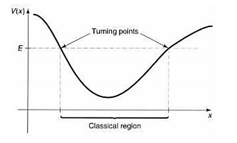
The classical turning point is defined as the point at which the potential energy \(U\) is approximately equal to total energy \(E\) \((U \approx E)\) and the kinetic energy equals zero. This occurs because the mass stops and reverses its velocity is zero. It is an inflection point that marks the boundaries between regions where a classical particle is allowed and where it is not, as well as where two wavefunctions must be properly matched.
If \(E > U\), a classical particle has a non-zero kinetic energy and is allowed to move freely. If \(U\) is a constant, the solution to the one-dimensional Schrödinger equation is:
\[\psi(x)=Ae^{\pm ikx},\label{56.3} \]
in which the wavefunction is oscillatory with constant wavelength λ and constant amplitude A. \(k(x)\) is defined as:
\[k(x)=\sqrt{\dfrac{2m(E-U(x))}{\hbar^2}}\label{56.4} \]
If \(E < U\), the solution to the Schrödinger equation for a constant \(U\) is:
\[\psi(x)=Ae^{\pm\kappa x}. \label{56.5} \]
In these regions, a classical particle would not be allowed, but there is a finite probability that a particle can pass through a potential energy barrier in quantum mechanics. The quantum particle is described as ‘tunnelling’, which is important in determining the rates of chemical reactions, particularly at lower temperatures. \(k(x)\) is defined as:
\[k(x)=-i\sqrt{\dfrac{2m(U(x)-E)}{\hbar^2}} = -i\kappa(x).\label{56.6} \]
If \(U(x)\) is not a constant, but instead varies very slowly on a distance scale of \(λ\), then it is reasonable to suppose that ψ remains practically sinusoidal, except that the wavelength and amplitude change slowly with \(x\).
WKB Approximation
Substituting in the normalized version of Equation \ref{56.2}, the Schrödinger Equation:
\[\dfrac{-\hbar^2}{2m}\dfrac{\partial^2}{\partial x^2}\psi(x)+U(x)\psi(x)=E\psi(x)\label{56.7} \]
becomes
\[i\dfrac{\partial^2\phi}{\partial x^2}-\left(\dfrac{\partial\phi}{\partial x}\right)^2+(k(x))^2=0.\label{56.8} \]
The WKB Approximation assumes that the potentials, \(k(x)\) and \(\phi (x)\) are slowly varying.
The 0th order WKB Approximation assumes:
\[\dfrac{\partial^2\phi}{\partial x^2} \ge 0.\label{56.9}\]
Thus,
\[\left(\dfrac{\partial\phi_0}{\partial x}\right)^2=(k(x))^2\label{56.10} \]
Solving,
\[\phi_0(x)=\pm\int k(x)dx+C_0\label{56.11} \]
and substituting \(\phi_0(x)\) into Equation \ref{56.2},
\[\psi(x)=e^{i(\pm\int k(x)dx+C_0)}.\label{56.12} \]
To obtain a more accurate solution, we manipulate Equation \ref{56.8} to solve for \(\phi(x)\).
\[i\dfrac{\partial^2\phi}{\partial x^2}-\left(\dfrac{\partial\phi}{\partial x}\right)^2+(k(x))^2=0 \nonumber \]
\[\left(\dfrac{\partial\phi}{\partial x}\right)^2=(k(x))^2+i\dfrac{\partial^2\phi}{\partial x^2} \nonumber \]
\[\dfrac{\partial\phi}{\partial x}=\sqrt{(k(x))^2+i\dfrac{\partial^2\phi}{\partial x^2}} \nonumber \]
So,
\[\phi(x)=\pm\int\sqrt{(k(x))^2+i\dfrac{\partial^2\phi}{\partial x^2}}dx+C_1\label{56.13} \]
The 1st order WKB Approximation follows the assumption of Equation \ref{56.10} from the 0th order solution. Taking its square root, we find that:
\[\dfrac{\partial\phi_0}{\partial x}=\pm k(x).\label{56.14} \]
Taking the derivative on both sides with respect to \(x\), we find that:
\[\dfrac{\partial^2\phi_0}{\partial x^2}=\pm \dfrac{\partial}{\partial x}k(x).\label{56.15} \]
Solving,
\[\phi_1(x)=\pm\int\sqrt{(k(x))^2\pm i\dfrac{\partial}{\partial x}k(x)}dx+C_1\label{56.16} \]
and substituting \(\phi_1(x)\) into Equation \ref{56.2},
\[\psi(x)=e^{i\left( \pm\int\sqrt{(k(x))^2\pm i\dfrac{\partial}{\partial x}k(x)}dx+C_1\right)}.\label{56.17} \]
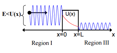
Determine the tunneling probability \(T\) at a finite width potential barrier.
Solution
Given:
\[T = \dfrac{\psi^*(L) \psi(L)}{\psi^*(0)\psi(0)} \nonumber \]
where
\[\psi(x)=\psi(0)e^{i\pm(\int k(x)dx+C_1)} \nonumber \]
For tunneling to occur, \(E < U\). So,
\(k(x)=-i\sqrt{\dfrac{2m(U(x)-E)}{\hbar^2}}\) for \(E < U(x)\), assuming \(U(x) = U\).
Plugging in \(k(x)\) to solve for the wavefunction,
\[ \begin{align*} \psi(x) &=\psi(0)e^{i\left(\pm\int_{0}^{x}-i\sqrt{\dfrac{2m(U(x)-E)}{\hbar^2}}dx\right)} \\[4pt] &=\psi(0)e^{\left(-\int_{0}^{x}\sqrt{\dfrac{2m(U-E)}{\hbar^2}}dx\right)} \\[4pt] &=\psi(0)e^{\left(-\left(\sqrt{\dfrac{2m(U-E)}{\hbar^2}}\right)x\right)} \end{align*} \]
Thus solving for the the tunneling probability \(T\),
\[ \begin{align*} T &= \dfrac{\psi^*(L) \psi(L)}{\psi^*(0)\psi(0)} \\[4pt] &= \dfrac{\psi(0)e^{\left( - \left( \sqrt{\dfrac{2m(U-E)}{\hbar^2}}\right) L \right)} \psi(0)e^{\left( - \left( \sqrt{\dfrac{2m(U-E)}{\hbar^2}}\right) L \right)}}{\psi(0)e^{\left( - \left( \sqrt{\dfrac{2m(U-E)}{\hbar^2}}\right) 0 \right)} \psi(0)e^{\left( - \left( \sqrt{\dfrac{2m(U-E)}{\hbar^2}}\right) 0 \right)}} \\[4pt] &= e^{\left( -2 \left( \sqrt{\dfrac{2m(U-E)}{\hbar^2}}\right) L \right)} \end{align*} \]