10.21: Variation Calculation on the 1D Hydrogen Atom Using a Trigonometric Trial Wave Function
- Page ID
- 136970

\( \newcommand{\vecs}[1]{\overset { \scriptstyle \rightharpoonup} {\mathbf{#1}} } \)
\( \newcommand{\vecd}[1]{\overset{-\!-\!\rightharpoonup}{\vphantom{a}\smash {#1}}} \)
\( \newcommand{\id}{\mathrm{id}}\) \( \newcommand{\Span}{\mathrm{span}}\)
( \newcommand{\kernel}{\mathrm{null}\,}\) \( \newcommand{\range}{\mathrm{range}\,}\)
\( \newcommand{\RealPart}{\mathrm{Re}}\) \( \newcommand{\ImaginaryPart}{\mathrm{Im}}\)
\( \newcommand{\Argument}{\mathrm{Arg}}\) \( \newcommand{\norm}[1]{\| #1 \|}\)
\( \newcommand{\inner}[2]{\langle #1, #2 \rangle}\)
\( \newcommand{\Span}{\mathrm{span}}\)
\( \newcommand{\id}{\mathrm{id}}\)
\( \newcommand{\Span}{\mathrm{span}}\)
\( \newcommand{\kernel}{\mathrm{null}\,}\)
\( \newcommand{\range}{\mathrm{range}\,}\)
\( \newcommand{\RealPart}{\mathrm{Re}}\)
\( \newcommand{\ImaginaryPart}{\mathrm{Im}}\)
\( \newcommand{\Argument}{\mathrm{Arg}}\)
\( \newcommand{\norm}[1]{\| #1 \|}\)
\( \newcommand{\inner}[2]{\langle #1, #2 \rangle}\)
\( \newcommand{\Span}{\mathrm{span}}\) \( \newcommand{\AA}{\unicode[.8,0]{x212B}}\)
\( \newcommand{\vectorA}[1]{\vec{#1}} % arrow\)
\( \newcommand{\vectorAt}[1]{\vec{\text{#1}}} % arrow\)
\( \newcommand{\vectorB}[1]{\overset { \scriptstyle \rightharpoonup} {\mathbf{#1}} } \)
\( \newcommand{\vectorC}[1]{\textbf{#1}} \)
\( \newcommand{\vectorD}[1]{\overrightarrow{#1}} \)
\( \newcommand{\vectorDt}[1]{\overrightarrow{\text{#1}}} \)
\( \newcommand{\vectE}[1]{\overset{-\!-\!\rightharpoonup}{\vphantom{a}\smash{\mathbf {#1}}}} \)
\( \newcommand{\vecs}[1]{\overset { \scriptstyle \rightharpoonup} {\mathbf{#1}} } \)
\( \newcommand{\vecd}[1]{\overset{-\!-\!\rightharpoonup}{\vphantom{a}\smash {#1}}} \)
\(\newcommand{\avec}{\mathbf a}\) \(\newcommand{\bvec}{\mathbf b}\) \(\newcommand{\cvec}{\mathbf c}\) \(\newcommand{\dvec}{\mathbf d}\) \(\newcommand{\dtil}{\widetilde{\mathbf d}}\) \(\newcommand{\evec}{\mathbf e}\) \(\newcommand{\fvec}{\mathbf f}\) \(\newcommand{\nvec}{\mathbf n}\) \(\newcommand{\pvec}{\mathbf p}\) \(\newcommand{\qvec}{\mathbf q}\) \(\newcommand{\svec}{\mathbf s}\) \(\newcommand{\tvec}{\mathbf t}\) \(\newcommand{\uvec}{\mathbf u}\) \(\newcommand{\vvec}{\mathbf v}\) \(\newcommand{\wvec}{\mathbf w}\) \(\newcommand{\xvec}{\mathbf x}\) \(\newcommand{\yvec}{\mathbf y}\) \(\newcommand{\zvec}{\mathbf z}\) \(\newcommand{\rvec}{\mathbf r}\) \(\newcommand{\mvec}{\mathbf m}\) \(\newcommand{\zerovec}{\mathbf 0}\) \(\newcommand{\onevec}{\mathbf 1}\) \(\newcommand{\real}{\mathbb R}\) \(\newcommand{\twovec}[2]{\left[\begin{array}{r}#1 \\ #2 \end{array}\right]}\) \(\newcommand{\ctwovec}[2]{\left[\begin{array}{c}#1 \\ #2 \end{array}\right]}\) \(\newcommand{\threevec}[3]{\left[\begin{array}{r}#1 \\ #2 \\ #3 \end{array}\right]}\) \(\newcommand{\cthreevec}[3]{\left[\begin{array}{c}#1 \\ #2 \\ #3 \end{array}\right]}\) \(\newcommand{\fourvec}[4]{\left[\begin{array}{r}#1 \\ #2 \\ #3 \\ #4 \end{array}\right]}\) \(\newcommand{\cfourvec}[4]{\left[\begin{array}{c}#1 \\ #2 \\ #3 \\ #4 \end{array}\right]}\) \(\newcommand{\fivevec}[5]{\left[\begin{array}{r}#1 \\ #2 \\ #3 \\ #4 \\ #5 \\ \end{array}\right]}\) \(\newcommand{\cfivevec}[5]{\left[\begin{array}{c}#1 \\ #2 \\ #3 \\ #4 \\ #5 \\ \end{array}\right]}\) \(\newcommand{\mattwo}[4]{\left[\begin{array}{rr}#1 \amp #2 \\ #3 \amp #4 \\ \end{array}\right]}\) \(\newcommand{\laspan}[1]{\text{Span}\{#1\}}\) \(\newcommand{\bcal}{\cal B}\) \(\newcommand{\ccal}{\cal C}\) \(\newcommand{\scal}{\cal S}\) \(\newcommand{\wcal}{\cal W}\) \(\newcommand{\ecal}{\cal E}\) \(\newcommand{\coords}[2]{\left\{#1\right\}_{#2}}\) \(\newcommand{\gray}[1]{\color{gray}{#1}}\) \(\newcommand{\lgray}[1]{\color{lightgray}{#1}}\) \(\newcommand{\rank}{\operatorname{rank}}\) \(\newcommand{\row}{\text{Row}}\) \(\newcommand{\col}{\text{Col}}\) \(\renewcommand{\row}{\text{Row}}\) \(\newcommand{\nul}{\text{Nul}}\) \(\newcommand{\var}{\text{Var}}\) \(\newcommand{\corr}{\text{corr}}\) \(\newcommand{\len}[1]{\left|#1\right|}\) \(\newcommand{\bbar}{\overline{\bvec}}\) \(\newcommand{\bhat}{\widehat{\bvec}}\) \(\newcommand{\bperp}{\bvec^\perp}\) \(\newcommand{\xhat}{\widehat{\xvec}}\) \(\newcommand{\vhat}{\widehat{\vvec}}\) \(\newcommand{\uhat}{\widehat{\uvec}}\) \(\newcommand{\what}{\widehat{\wvec}}\) \(\newcommand{\Sighat}{\widehat{\Sigma}}\) \(\newcommand{\lt}{<}\) \(\newcommand{\gt}{>}\) \(\newcommand{\amp}{&}\) \(\definecolor{fillinmathshade}{gray}{0.9}\)The energy operator for this problem is:
\[ \frac{-1}{2} \frac{d^2}{dx^2} \blacksquare - \frac{1}{x} \blacksquare \nonumber \]
The trial wave function:
\[ \Psi ( \alpha , x) := \frac{ \sqrt{12 \alpha ^3}}{ \pi} (x) sech( \alpha , x) \nonumber \]
Evaluate the variational energy integral.
\[ E( \alpha ) := \int_{0}^{ \infty} \Psi ( \alpha , x) - \frac{1}{2} \frac{d^2}{dx^2} \Psi ( \alpha , x) dx + \int_{0}^{ \infty} \frac{-1}{x} \Psi ( \alpha , x)^2 dx |_{simplify}^{assume,~ \alpha > 0} \rightarrow \frac{1}{6} \alpha \frac{12 \alpha _ \alpha \pi^2 - 72 ln (2)}{ \pi ^2} \nonumber \]
Minimize the energy with respect to the variational parameter \( \alpha\) and report its optimum value and the ground-state energy.
\( \alpha\) := 1 \( \alpha\) := Minimize (E, \( \alpha\)) \( \alpha\) = 1.1410 E( \( \alpha\)) = -0.4808
The exact ground-state energy for the hydrogen atom is -.5 Eh. Calculate the percent error.
\[ | \frac{-.5 - E( \alpha )}{-.5}| = 3.8401 \nonumber \]
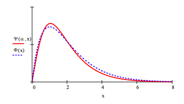
Plot the optimized trial wave function and the exact solution, \( \Phi (x) := 2 (x) exp (-x)\).
Find the distance from the nucleus within which there is a 95% probability of finding the electron.
\( \alpha\) := 1. Given:
\[ \int_{0}^{a} \Psi ( \alpha , x)^2 dx = 0.95 \nonumber \]
Find (a) = 2.8754
Find the most probable value of the position of the electron from the nucleus.
\[ \alpha := 1.1410~~~~ \frac{d}{dx}|\frac{ \sqrt{12 \alpha ^3}}{ \pi} (x) sech( \alpha , x)| = 0~|_{float,~3}^{solve,~x} \rightarrow 1.05 \nonumber \]
Calculate the probability that the electron will be found between the nucleus and the most probable distance from the nucleus.
\[ \int_{0}^{1.05} \Psi ( \alpha , x)^2 dx = 0.3464 \nonumber \]
Break the energy down into kinetic and potential energy contributions. Is the virial theorem obeyed?
\[ T := \int_{0}^{ \infty} \Psi ( \alpha , x) \frac{-1}{2} \frac{d^2}{dx^2} \Psi ( \alpha , x) dx~~~T = 0.4808 \nonumber \]
\[ V := \int_{0}^{ \infty} \frac{-1}{x} \Psi ( \alpha , x)^2 dx~~~ V = -0.9616 \nonumber \]
\[ | \frac{V}{T}| = 2.0000 \nonumber \]
Use the exact result to discuss the weakness of this trial function.
Eexact := -0.5
Using the virial theorem we know: Texact := 0.500 Vexact := -1.00
Calculate the difference between the variational results and the exact calculation:
E( \( \alpha\)) - Eexact = 0.0192
T - Texact = -0.0192
V - Vexact = 0.0384
The variational wave function yields a lower kinetic energy, but at the expense of a potential energy that is twice as unfavorable as the kinetic energy result is favorable.
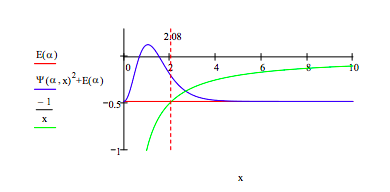
Calculate the probability that tunneling is occurring.
Classical turning point:
\[ E( \alpha ) = \frac{-1}{x} |_{float,~3}^{solve,~x} \nonumber \]
Tunneling probability:
\[ \int_{2.08}^{ \infty} \Psi ( \alpha , x)^2 dx = 0.1783 \nonumber \]