10.20: Gaussian Trial Wavefunction for the Hydrogen Atom
- Page ID
- 136259

\( \newcommand{\vecs}[1]{\overset { \scriptstyle \rightharpoonup} {\mathbf{#1}} } \)
\( \newcommand{\vecd}[1]{\overset{-\!-\!\rightharpoonup}{\vphantom{a}\smash {#1}}} \)
\( \newcommand{\id}{\mathrm{id}}\) \( \newcommand{\Span}{\mathrm{span}}\)
( \newcommand{\kernel}{\mathrm{null}\,}\) \( \newcommand{\range}{\mathrm{range}\,}\)
\( \newcommand{\RealPart}{\mathrm{Re}}\) \( \newcommand{\ImaginaryPart}{\mathrm{Im}}\)
\( \newcommand{\Argument}{\mathrm{Arg}}\) \( \newcommand{\norm}[1]{\| #1 \|}\)
\( \newcommand{\inner}[2]{\langle #1, #2 \rangle}\)
\( \newcommand{\Span}{\mathrm{span}}\)
\( \newcommand{\id}{\mathrm{id}}\)
\( \newcommand{\Span}{\mathrm{span}}\)
\( \newcommand{\kernel}{\mathrm{null}\,}\)
\( \newcommand{\range}{\mathrm{range}\,}\)
\( \newcommand{\RealPart}{\mathrm{Re}}\)
\( \newcommand{\ImaginaryPart}{\mathrm{Im}}\)
\( \newcommand{\Argument}{\mathrm{Arg}}\)
\( \newcommand{\norm}[1]{\| #1 \|}\)
\( \newcommand{\inner}[2]{\langle #1, #2 \rangle}\)
\( \newcommand{\Span}{\mathrm{span}}\) \( \newcommand{\AA}{\unicode[.8,0]{x212B}}\)
\( \newcommand{\vectorA}[1]{\vec{#1}} % arrow\)
\( \newcommand{\vectorAt}[1]{\vec{\text{#1}}} % arrow\)
\( \newcommand{\vectorB}[1]{\overset { \scriptstyle \rightharpoonup} {\mathbf{#1}} } \)
\( \newcommand{\vectorC}[1]{\textbf{#1}} \)
\( \newcommand{\vectorD}[1]{\overrightarrow{#1}} \)
\( \newcommand{\vectorDt}[1]{\overrightarrow{\text{#1}}} \)
\( \newcommand{\vectE}[1]{\overset{-\!-\!\rightharpoonup}{\vphantom{a}\smash{\mathbf {#1}}}} \)
\( \newcommand{\vecs}[1]{\overset { \scriptstyle \rightharpoonup} {\mathbf{#1}} } \)
\( \newcommand{\vecd}[1]{\overset{-\!-\!\rightharpoonup}{\vphantom{a}\smash {#1}}} \)
\(\newcommand{\avec}{\mathbf a}\) \(\newcommand{\bvec}{\mathbf b}\) \(\newcommand{\cvec}{\mathbf c}\) \(\newcommand{\dvec}{\mathbf d}\) \(\newcommand{\dtil}{\widetilde{\mathbf d}}\) \(\newcommand{\evec}{\mathbf e}\) \(\newcommand{\fvec}{\mathbf f}\) \(\newcommand{\nvec}{\mathbf n}\) \(\newcommand{\pvec}{\mathbf p}\) \(\newcommand{\qvec}{\mathbf q}\) \(\newcommand{\svec}{\mathbf s}\) \(\newcommand{\tvec}{\mathbf t}\) \(\newcommand{\uvec}{\mathbf u}\) \(\newcommand{\vvec}{\mathbf v}\) \(\newcommand{\wvec}{\mathbf w}\) \(\newcommand{\xvec}{\mathbf x}\) \(\newcommand{\yvec}{\mathbf y}\) \(\newcommand{\zvec}{\mathbf z}\) \(\newcommand{\rvec}{\mathbf r}\) \(\newcommand{\mvec}{\mathbf m}\) \(\newcommand{\zerovec}{\mathbf 0}\) \(\newcommand{\onevec}{\mathbf 1}\) \(\newcommand{\real}{\mathbb R}\) \(\newcommand{\twovec}[2]{\left[\begin{array}{r}#1 \\ #2 \end{array}\right]}\) \(\newcommand{\ctwovec}[2]{\left[\begin{array}{c}#1 \\ #2 \end{array}\right]}\) \(\newcommand{\threevec}[3]{\left[\begin{array}{r}#1 \\ #2 \\ #3 \end{array}\right]}\) \(\newcommand{\cthreevec}[3]{\left[\begin{array}{c}#1 \\ #2 \\ #3 \end{array}\right]}\) \(\newcommand{\fourvec}[4]{\left[\begin{array}{r}#1 \\ #2 \\ #3 \\ #4 \end{array}\right]}\) \(\newcommand{\cfourvec}[4]{\left[\begin{array}{c}#1 \\ #2 \\ #3 \\ #4 \end{array}\right]}\) \(\newcommand{\fivevec}[5]{\left[\begin{array}{r}#1 \\ #2 \\ #3 \\ #4 \\ #5 \\ \end{array}\right]}\) \(\newcommand{\cfivevec}[5]{\left[\begin{array}{c}#1 \\ #2 \\ #3 \\ #4 \\ #5 \\ \end{array}\right]}\) \(\newcommand{\mattwo}[4]{\left[\begin{array}{rr}#1 \amp #2 \\ #3 \amp #4 \\ \end{array}\right]}\) \(\newcommand{\laspan}[1]{\text{Span}\{#1\}}\) \(\newcommand{\bcal}{\cal B}\) \(\newcommand{\ccal}{\cal C}\) \(\newcommand{\scal}{\cal S}\) \(\newcommand{\wcal}{\cal W}\) \(\newcommand{\ecal}{\cal E}\) \(\newcommand{\coords}[2]{\left\{#1\right\}_{#2}}\) \(\newcommand{\gray}[1]{\color{gray}{#1}}\) \(\newcommand{\lgray}[1]{\color{lightgray}{#1}}\) \(\newcommand{\rank}{\operatorname{rank}}\) \(\newcommand{\row}{\text{Row}}\) \(\newcommand{\col}{\text{Col}}\) \(\renewcommand{\row}{\text{Row}}\) \(\newcommand{\nul}{\text{Nul}}\) \(\newcommand{\var}{\text{Var}}\) \(\newcommand{\corr}{\text{corr}}\) \(\newcommand{\len}[1]{\left|#1\right|}\) \(\newcommand{\bbar}{\overline{\bvec}}\) \(\newcommand{\bhat}{\widehat{\bvec}}\) \(\newcommand{\bperp}{\bvec^\perp}\) \(\newcommand{\xhat}{\widehat{\xvec}}\) \(\newcommand{\vhat}{\widehat{\vvec}}\) \(\newcommand{\uhat}{\widehat{\uvec}}\) \(\newcommand{\what}{\widehat{\wvec}}\) \(\newcommand{\Sighat}{\widehat{\Sigma}}\) \(\newcommand{\lt}{<}\) \(\newcommand{\gt}{>}\) \(\newcommand{\amp}{&}\) \(\definecolor{fillinmathshade}{gray}{0.9}\)A Gaussian function, exp(‐αr2), is proposed as a trial wavefunction in a variational calculation on the hydrogen atom. Determine the optimum value of the parameter α and the ground state energy of the hydrogen atom. Use atomic units: h = 2π, me = 1, e = ‐1.
\[ \Phi (r, \beta ) := ( \frac{2 \beta}{ \pi})^{ \frac{3}{4}} exp(- \beta r^2) \nonumber \]
\[ T = \frac{-1}{2r} \frac{d^2}{dr^2} (r \blacksquare ) \nonumber \]
\[ V = \frac{1}{r} \nonumber \]
\[ \int_{0}^{ \infty} \blacksquare 4 \pi r^2 dr \nonumber \]
a. Demonstrate the wave function is normalized.
\[ \int_{0}^{ \infty} \Psi (r, \beta )^2 4 \pi r^2 dr |_{simplify}^{assume,~ \beta >0} \rightarrow 1 \nonumber \]
b. Evaluate the variational integral.
\[ E ( \beta ) := \int_{0}^{ \infty} \Psi (r, \beta ) [ \frac{-1}{2r} \frac{d^2}{dr^2} (r \Psi (r, \beta ))] 4 \pi r^2 dr ... |_{simplify}^{assume,~ \beta >0} \rightarrow \frac{1}{2} \frac{3 \pi^{\frac{1}{2}} \beta - (4) 2^{ \frac{1}{2}} \beta^{ \frac{1}{2}}}{ \pi^{ \frac{1}{2}}} + \int_{0}^{ \infty} \Psi (r, \beta ) \frac{-1}{r} \Psi (r, \beta ) 4 \pi r^2 dr \nonumber \]
c. Minimize the energy with respect to the variational parameter \( \beta\).
\( \beta\) := 1 \( \beta\) := Minimize (E, \( \beta\)) \( \beta\) = 0.283 E( \( \beta\)) = -0.424
d. The exact ground state energy for the hydrogen atom is -.5 Eh. Calculate the percent error.
\[ \frac{-.5 - E( \beta )}{-.5} = 15.117 \nonumber \]
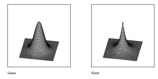
e. The differences between the Gaussian and Slate type wavefunctions are illustrated with the surface plots shown below.
N := 50 b := 5 i := 0..N j := 0..N \( y_{i} := -b + \frac{2bi}{N}\) \( x_{j} := -b + \frac{2bj}{N}\)
\[ Gauss_{i,~j} := ( \frac{2 \beta}{ \pi})^{ \frac{3}{4}} exp[- \beta [ (x_{i})^2 + (y_{j})^2]] \nonumber \]
\[ Slater_{i,~j} := \frac{1}{ \sqrt{ \pi}} exp [ - \sqrt{ (x_{i})^2 + (y_{j})^2}] \nonumber \]
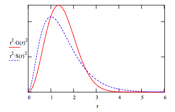
f. These wavefunctions can also be compared to their radial distribution functions:
r := 0, .1 .. 6
\[ G(r) := ( \frac{2 \beta}{ \pi}) ^{ \frac{3}{4}} exp( - \beta r^2) \nonumber \]
\[ S(r) := \frac{1}{ \sqrt{ \pi}} exp( -r ) \nonumber \]