8.47: Another Bell Theorem Analysis

The purpose of this tutorial is to review Jim Baggott's analysis of Bell's theorem as presented in Chapter 4 of The Meaning of Quantum Theory using matrix and tensor algebra.

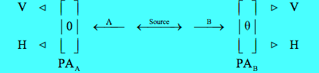
A two-stage atomic cascade emits entangled photons (A and B) in opposite directions with the same circular polarization according to observers in their path.

\[ | \Psi \rangle = \frac{1}{ \sqrt{2}} \left[ |L \rangle_A |L \rangle_B + |R \rangle_A |R \rangle_B \right] \nonumber \]

The experiment involves the measurement of photon polarization states in the vertical/horizontal measurement basis, and allows for the rotation of the right-hand detector through an angle of θ, in order to explore the consequences of quantum mechanical entanglement. PA stands for polarization analyzer and could simply be a calcite crystal.

In vector notation the left- and right-circular polarization states are expressed as follows:

Left circular polarization:

\[ L = \frac{1}{ \sqrt{2}} \begin{pmatrix} 1 \\ i \end{pmatrix} \nonumber \]

Right circular polarization:

\[ R = \frac{1}{ \sqrt{2}} \begin{pmatrix} 1 \\ -i \end{pmatrix} \nonumber \]

In tensor notation the initial state is the following entangled superposition,

\[ | \Psi \rangle = \frac{1}{ \sqrt{2}} \left[ | L \rangle_A | L \rangle_B + |R \rangle_A | R \rangle_B \right] = \frac{1}{ 2 \sqrt{2}} \left[ \begin{pmatrix} 1 \\ i \end{pmatrix}_A \otimes \begin{pmatrix} 1 \\ i \end{pmatrix}_B + \begin{pmatrix} 1 \\ -i \end{pmatrix}_A \otimes \begin{pmatrix} 1 \\ -i \end{pmatrix}_B \right] = \frac{1}{2 \sqrt{2}} \left[ \begin{pmatrix} 1 \\ i \\ i \\ -1 \end{pmatrix} + \begin{pmatrix} 1 \\ -i \\ -i \\ -1 \end{pmatrix} \right] = \frac{1}{ \sqrt{2}} \begin{pmatrix} 1 \\ 0 \\ 0 \\ -1 \end{pmatrix} \nonumber \]

However, as mentioned above, the photon polarization measurements will actually be made in the vertical/horizontal basis. These polarization measurement states for photons A and B in vector representation are given below. Θ is the angle through which the PA₂ has been rotated.

Vertical polarization:

\[ \begin{matrix} V_A = \begin{pmatrix} 1 \\ 0 \end{pmatrix} & V_B = \begin{pmatrix} \cos \theta \\ - \sin \theta \end{pmatrix} \end{matrix} \nonumber \]

Horizontal polarization:

\[ \begin{matrix} V_A = \begin{pmatrix} 0 \\ 1 \end{pmatrix} & V_B = \begin{pmatrix} \sin \theta \\ \cos \theta \end{pmatrix} \end{matrix} \nonumber \]

It is easy to show that |Ψ> in the vertical/horizontal basis is,

\[ | \Psi \rangle = \frac{1}{ \sqrt{2}} \left[ | V \rangle_A | V \rangle_B + |H \rangle_A | H \rangle_B \right] = \frac{1}{ 2 \sqrt{2}} \left[ \begin{pmatrix} 1 \\ 0 \end{pmatrix}_A \otimes \begin{pmatrix} 1 \\ 0 \end{pmatrix}_B + \begin{pmatrix} 0 \\ 1 \end{pmatrix}_A \otimes \begin{pmatrix} 0 \\ 1 \end{pmatrix}_B \right] = \frac{1}{2 \sqrt{2}} \left[ \begin{pmatrix} 1 \\ 0 \\ 0 \\ 0 \end{pmatrix} + \begin{pmatrix} 0 \\ 0 \\ 0 \\ 1 \end{pmatrix} \right] = \frac{1}{ \sqrt{2}} \begin{pmatrix} 1 \\ 0 \\ 0 \\ -1 \end{pmatrix} \nonumber \]

There are four possible measurement outcomes: both photons are vertically polarized, both are horizontally polarized, one is vertical and the other horizontal, and vice versa. The vector representations of the measurement states are obtained by tensor multiplication of the individual photon states.

\[ \begin{matrix} | V_A V_B \rangle = \begin{pmatrix} 1 \\ 0 \end{pmatrix} \otimes \begin{pmatrix} \cos \theta \\ - \sin \theta \end{pmatrix} = \begin{pmatrix} \cos \theta \\ - \sin \theta \\ 0 \\ 0 \end{pmatrix} & | V_A H_B \rangle = \begin{pmatrix} 1 \\ 0 \end{pmatrix} \otimes \begin{pmatrix} \sin \theta \\ \cos \theta \end{pmatrix} = \begin{pmatrix} \sin \theta \\ \cos \theta \\ 0 \\ 0 \end{pmatrix} \\ | H_A V_B \rangle = \begin{pmatrix} 0 \\ 1 \end{pmatrix} \otimes \begin{pmatrix} \cos \theta \\ - \sin \theta \end{pmatrix} = \begin{pmatrix} 0 \\ 0 \\ \cos \theta \\ - \sin \theta \end{pmatrix} & | H_A H_B \rangle = \begin{pmatrix} 0 \\ 1 \end{pmatrix} \otimes \begin{pmatrix} \sin \theta \\ \cos \theta \end{pmatrix} = \begin{pmatrix} 0 \\ 0 \\ \sin \theta \\ \cos \theta \end{pmatrix} \end{matrix} \nonumber \]

The initial state and the measurement eigenstates are written in Mathcad syntax.

\[ \begin{matrix} \Psi = \frac{1}{ \sqrt{2}} \begin{pmatrix} 1 \\ 0 \\ 0 \\ -1 \end{pmatrix} & V_a V_b ( \theta) = \begin{pmatrix} \cos \theta \\ - \sin \theta \\ 0 \\ 0 \end{pmatrix} & V_a H_b ( \theta) = \begin{pmatrix} \sin \theta \\ \cos \theta \\ 0 \\ 0 \end{pmatrix} \\ ~ & H_a V_b ( \theta) = \begin{pmatrix} 0 \\ 0 \\ \cos ( \theta) \\ - \sin ( \theta) \end{pmatrix} & H_a H_b ( \theta) = \begin{pmatrix} 0 \\ 0 \\ \sin ( \theta) \\ \cos ( \theta) \end{pmatrix} \end{matrix} \nonumber \]

The projections of the initial state onto the four measurement states are,

Probability amplitude:

\[ \begin{pmatrix} V_a V_b ( \theta)^T \Psi \\ V_a H_b ( \theta)^T \Psi \\ H_a V_b ( \theta)^T \Psi \\ H_a H_b ( \theta)^T \Psi \end{pmatrix} \rightarrow \begin{pmatrix} \frac{ \sqrt{2} \cos ( \theta)}{2} \\ \frac{ \sqrt{2} \sin ( \theta)}{2} \\ \frac{ \sqrt{2} \sin ( \theta)}{2} \\ \frac{ \sqrt{2} \cos ( \theta)}{2} \end{pmatrix} \nonumber \]

Probability:

\[ \begin{bmatrix} \left( V_a V_b ( \theta)^T \Psi \right)^2 \\ \left( V_a H_b ( \theta)^T \Psi \right)^2 \\ \left( H_a V_b ( \theta)^T \Psi \right)^2 \\ \left( H_a H_b ( \theta)^T \Psi \right)^2 \end{bmatrix} \rightarrow \begin{pmatrix} \frac{ \cos ( \theta)^2}{2} \\ \frac{ \sin ( \theta)^2}{2} \\ \frac{ \sin ( \theta)^2}{2} \\ \frac{ \cos ( \theta)^2}{2} \end{pmatrix} \nonumber \]

Assigning an eigenvalue of +1 to a vertical polarization measurement and -1 to a horizontal polarization measurement allows the calculation of the expectation value for the joint polarization measurements, a function which quantifies the correlation between the joint measurements. The eigenvalues for the four joint measurement outcomes are: V_aV_b = 1; V_aH_b = -1; H_aV_b = -1; H_aH_b = 1. Weighting these by the probability of their occurence gives the expectation value or correlation function.

\[ E( \theta) = \left( V_a V_b ( \theta)^T \Psi \right)^2 - \left( V_a H_b ( \theta)^T \Psi \right)^2 - \left( H_a V_b ( \theta)^T \Psi \right)^2 + \left( H_a H_b ( \theta)^T \Psi \right)^2 ~ \text{simplify} \rightarrow \cos (2 \theta) \nonumber \]

As shown above the evaluation of E(θ) yields cos(2θ). For θ = 0⁰ there is perfect correlation; for θ = 90⁰ perfect anti-correlation; for θ = 45⁰ no correlation.

\[ \begin{matrix} E \text{(0 deg)} = 1 & E \text{(90 deg)} = -1 & E \text{(45 deg)} = 0 \end{matrix} \nonumber \]

Baggott presented a correlation function for this experiment based on a local hidden variable model of reality (pp. 110-113, 127-131). It (linear blue line) and the quantum mechanical correlation function, E(θ), are compared on the graph below. Quantum theory and local realism disagree at all angles except 0, 45 and 90 degrees.

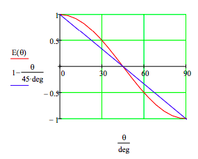
This example illustrates Bell's theorem: no local hidden-variable theory can reproduce all the predictions of quantum mechanics for entangled composite systems. As the quantum predictions are confirmed experimentally, the local hidden-variable approach to reality must be abandoned.

Appendix

An equivalent computational approach creates a joint measurement operator from the A and B photon measurement eigenstates. This operator is then used to calculate the expectation value or correlation function.

\[ \left( V_A V_A^T - H_A H_A^T \right) \otimes \left( V_B V_B^T - H_B H_B^T \right) = \begin{pmatrix} 1 & 0 \\ 0 & -1 \end{pmatrix} \otimes \begin{pmatrix} \cos (2 \theta) & - \sin ( 2 \theta) \\ - \sin (2 \theta) & 2 \sin ( \theta)^2 - 1 \end{pmatrix} \nonumber \]

Recalling that the vertical and horizontal measurement eigenvalues are +1 and -1, the mathematical structures of the A and B operators shown above are confirmed.

\[ \begin{matrix} V_A V_A^T - H_A H_A^T \rightarrow \begin{pmatrix} 1 & 0 \\ 0 & -1 \end{pmatrix} & V_B V_B^T - H_B H_B^T ~ \text{simplify} \rightarrow \begin{pmatrix} \cos (2 \theta) & - \sin ( 2 \theta) \\ - \sin (2 \theta) & 2 \sin ( \theta)^2 - 1 \end{pmatrix} \end{matrix} \nonumber \]

Tensor multiplication of the individual operators creates the joint measurement operator used in the calculation below.

\[ E ( \theta ) = \Psi^T \begin{pmatrix} \cos (2 \theta) & - \sin (2 \theta) & 0 & 0 \\ - \sin (2 \theta) & 2 \sin ( \theta)^2 - 1 & 0 & 0 \\ 0 & 0 & - \cos(2 \theta) & \sin (2 \theta) \\ 0 & 0 & \sin (2 \theta) & 1 - 2 \sin ( \theta)^2 \end{pmatrix} ~ \text{simplify} ~ \rightarrow \cos (2 \theta) \nonumber \]

The expectation value calculations can also be performed using the trace function as shown below.

\[ \langle \Psi | \hat{O} | i \rangle \langle i | \Psi \rangle = \sum_i \langle \Psi | \hat{O} | i \rangle \langle i | \Psi \rangle = \sum_i \langle i | \Psi \rangle \langle \Psi | \hat{O} | i \rangle = Trace \left( | \Psi \rangle \langle \Psi | \hat{O} \right) ~ \text{where} ~ \sum_i |i \rangle \langle i | = \text{Identity} \nonumber \]

\[ tr \begin{bmatrix} \Psi \Psi^T \begin{pmatrix} \cos (2 \theta) & - \sin (2 \theta) & 0 & 0 \\ - \sin (2 \theta) & 2 \sin ( \theta)^2 - 1 & 0 & 0 \\ 0 & 0 & - \cos(2 \theta) & \sin (2 \theta) \\ 0 & 0 & \sin (2 \theta) & 1 - 2 \sin ( \theta)^2 \end{pmatrix} \end{bmatrix} ~ \text{simplify} \rightarrow ~ \cos ( 2 \theta) \nonumber \]