7.11: Polarized Light and Quantum Superposition
- Page ID
- 138799
\( \newcommand{\vecs}[1]{\overset { \scriptstyle \rightharpoonup} {\mathbf{#1}} } \)
\( \newcommand{\vecd}[1]{\overset{-\!-\!\rightharpoonup}{\vphantom{a}\smash {#1}}} \)
\( \newcommand{\id}{\mathrm{id}}\) \( \newcommand{\Span}{\mathrm{span}}\)
( \newcommand{\kernel}{\mathrm{null}\,}\) \( \newcommand{\range}{\mathrm{range}\,}\)
\( \newcommand{\RealPart}{\mathrm{Re}}\) \( \newcommand{\ImaginaryPart}{\mathrm{Im}}\)
\( \newcommand{\Argument}{\mathrm{Arg}}\) \( \newcommand{\norm}[1]{\| #1 \|}\)
\( \newcommand{\inner}[2]{\langle #1, #2 \rangle}\)
\( \newcommand{\Span}{\mathrm{span}}\)
\( \newcommand{\id}{\mathrm{id}}\)
\( \newcommand{\Span}{\mathrm{span}}\)
\( \newcommand{\kernel}{\mathrm{null}\,}\)
\( \newcommand{\range}{\mathrm{range}\,}\)
\( \newcommand{\RealPart}{\mathrm{Re}}\)
\( \newcommand{\ImaginaryPart}{\mathrm{Im}}\)
\( \newcommand{\Argument}{\mathrm{Arg}}\)
\( \newcommand{\norm}[1]{\| #1 \|}\)
\( \newcommand{\inner}[2]{\langle #1, #2 \rangle}\)
\( \newcommand{\Span}{\mathrm{span}}\) \( \newcommand{\AA}{\unicode[.8,0]{x212B}}\)
\( \newcommand{\vectorA}[1]{\vec{#1}} % arrow\)
\( \newcommand{\vectorAt}[1]{\vec{\text{#1}}} % arrow\)
\( \newcommand{\vectorB}[1]{\overset { \scriptstyle \rightharpoonup} {\mathbf{#1}} } \)
\( \newcommand{\vectorC}[1]{\textbf{#1}} \)
\( \newcommand{\vectorD}[1]{\overrightarrow{#1}} \)
\( \newcommand{\vectorDt}[1]{\overrightarrow{\text{#1}}} \)
\( \newcommand{\vectE}[1]{\overset{-\!-\!\rightharpoonup}{\vphantom{a}\smash{\mathbf {#1}}}} \)
\( \newcommand{\vecs}[1]{\overset { \scriptstyle \rightharpoonup} {\mathbf{#1}} } \)
\( \newcommand{\vecd}[1]{\overset{-\!-\!\rightharpoonup}{\vphantom{a}\smash {#1}}} \)
\(\newcommand{\avec}{\mathbf a}\) \(\newcommand{\bvec}{\mathbf b}\) \(\newcommand{\cvec}{\mathbf c}\) \(\newcommand{\dvec}{\mathbf d}\) \(\newcommand{\dtil}{\widetilde{\mathbf d}}\) \(\newcommand{\evec}{\mathbf e}\) \(\newcommand{\fvec}{\mathbf f}\) \(\newcommand{\nvec}{\mathbf n}\) \(\newcommand{\pvec}{\mathbf p}\) \(\newcommand{\qvec}{\mathbf q}\) \(\newcommand{\svec}{\mathbf s}\) \(\newcommand{\tvec}{\mathbf t}\) \(\newcommand{\uvec}{\mathbf u}\) \(\newcommand{\vvec}{\mathbf v}\) \(\newcommand{\wvec}{\mathbf w}\) \(\newcommand{\xvec}{\mathbf x}\) \(\newcommand{\yvec}{\mathbf y}\) \(\newcommand{\zvec}{\mathbf z}\) \(\newcommand{\rvec}{\mathbf r}\) \(\newcommand{\mvec}{\mathbf m}\) \(\newcommand{\zerovec}{\mathbf 0}\) \(\newcommand{\onevec}{\mathbf 1}\) \(\newcommand{\real}{\mathbb R}\) \(\newcommand{\twovec}[2]{\left[\begin{array}{r}#1 \\ #2 \end{array}\right]}\) \(\newcommand{\ctwovec}[2]{\left[\begin{array}{c}#1 \\ #2 \end{array}\right]}\) \(\newcommand{\threevec}[3]{\left[\begin{array}{r}#1 \\ #2 \\ #3 \end{array}\right]}\) \(\newcommand{\cthreevec}[3]{\left[\begin{array}{c}#1 \\ #2 \\ #3 \end{array}\right]}\) \(\newcommand{\fourvec}[4]{\left[\begin{array}{r}#1 \\ #2 \\ #3 \\ #4 \end{array}\right]}\) \(\newcommand{\cfourvec}[4]{\left[\begin{array}{c}#1 \\ #2 \\ #3 \\ #4 \end{array}\right]}\) \(\newcommand{\fivevec}[5]{\left[\begin{array}{r}#1 \\ #2 \\ #3 \\ #4 \\ #5 \\ \end{array}\right]}\) \(\newcommand{\cfivevec}[5]{\left[\begin{array}{c}#1 \\ #2 \\ #3 \\ #4 \\ #5 \\ \end{array}\right]}\) \(\newcommand{\mattwo}[4]{\left[\begin{array}{rr}#1 \amp #2 \\ #3 \amp #4 \\ \end{array}\right]}\) \(\newcommand{\laspan}[1]{\text{Span}\{#1\}}\) \(\newcommand{\bcal}{\cal B}\) \(\newcommand{\ccal}{\cal C}\) \(\newcommand{\scal}{\cal S}\) \(\newcommand{\wcal}{\cal W}\) \(\newcommand{\ecal}{\cal E}\) \(\newcommand{\coords}[2]{\left\{#1\right\}_{#2}}\) \(\newcommand{\gray}[1]{\color{gray}{#1}}\) \(\newcommand{\lgray}[1]{\color{lightgray}{#1}}\) \(\newcommand{\rank}{\operatorname{rank}}\) \(\newcommand{\row}{\text{Row}}\) \(\newcommand{\col}{\text{Col}}\) \(\renewcommand{\row}{\text{Row}}\) \(\newcommand{\nul}{\text{Nul}}\) \(\newcommand{\var}{\text{Var}}\) \(\newcommand{\corr}{\text{corr}}\) \(\newcommand{\len}[1]{\left|#1\right|}\) \(\newcommand{\bbar}{\overline{\bvec}}\) \(\newcommand{\bhat}{\widehat{\bvec}}\) \(\newcommand{\bperp}{\bvec^\perp}\) \(\newcommand{\xhat}{\widehat{\xvec}}\) \(\newcommand{\vhat}{\widehat{\vvec}}\) \(\newcommand{\uhat}{\widehat{\uvec}}\) \(\newcommand{\what}{\widehat{\wvec}}\) \(\newcommand{\Sighat}{\widehat{\Sigma}}\) \(\newcommand{\lt}{<}\) \(\newcommand{\gt}{>}\) \(\newcommand{\amp}{&}\) \(\definecolor{fillinmathshade}{gray}{0.9}\)The superposition principle is a deep and difficult quantum mechanical concept. There is no classical analog to lean on in probing its meaning, because it is impossible to simulate it with classical models. And yet because it pervades quantum mechanics we must find ways to present it to students that have some probability of success in revealing its significance.
The title of the first chapter in Dirac’s famous treatise The Principles of Quantum Mechanics (Clarendon Press, Oxford) is The Principle of Superposition. On page 12 of the 4th edition he wrote,
The nature of the relationships which the superposition principle requires to exist between the states of any system is of a kind that cannot be explained in terms of familiar physical concepts. One cannot in the classical sense picture a system being partly in each of two states and see the equivalence of this to the system being completely in some other state. There is an entirely new idea involved, to which one must get accustomed and in terms of which one must proceed to build up an exact mathematical theory, without having any detailed classical picture.
Perhaps the easiest way to illustrate the superposition principle mathematically is with demonstrations using polarizing films. Suppose unpolarized light illuminates a polarizer oriented at 45o to the vertical creating a beam of diagonally polarized photons, \(|D \rangle\). If the diagonally polarized beam now illuminates a second polarizer oriented in the vertical or horizontal direction, 50% of the photons are transmitted.
The quantum mechanical explanation for these results is to write the wave function of a diagonally polarized photon as a superposition in the V‐H basis, \( \langle v | v \rangle = \langle H | H \rangle = 1; \langle v | H \rangle \langle H |V \rangle = 0\).
\[ |D \rangle = \frac{1}{ \sqrt{2}} \left[ |V \rangle + |H \rangle \right] \nonumber \]
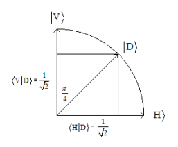
This superposition is illustrated graphically as follows.

Using either equation or figure we have, \( | \langle V |D \rangle |^2 = | \langle H | D \rangle |^2 = \frac{1}{2}\), in agreement with the demonstration.
The same result would occur if the diagonally polarized beam was assumed to be a 50‐ 50 mixture of vertical and horizontal photons rather than a superposition. However, according to quantum mechanical principles, a mixture is represented by a density operator rather than by a wave function. In this case the appropriate density operator is
\[ \hat{ \rho}_{mix} = \frac{1}{2} |V \rangle \langle V | + \frac{1}{2} |H \rangle \langle H| \nonumber \]
The probability (expectation value) that a 50‐50 mixture of V‐H photons will pass a vertical or horizontal polarizer is easily calculated.
\[ \langle V| \hat{ \rho}_{mix} |V \rangle = \langle H | \hat{ \rho}_{mix} |H \rangle = \frac{1}{2} \nonumber \]
At this point, the superposition and mixture models give the same result for what happens in the presence of the second (H or V) polarizer. However, it is not difficult to demonstrate that diagonally polarized light is not a mixture of vertical and horizontally polarized photons. If the second polarizer is replaced with another diagonally oriented polarizer, 100% of the photons are transmitted. This is because a diagonally polarized photon is an eigenstate of the diagonal polarization measurement operator.
The expectation value for a 50‐50 mixture is not in agreement with this outcome. It predicts that only 50% of the photons will pass the diagonal oriented polarizing film.
\[ \langle D | \hat{ \rho}_{mix} | D \rangle = \frac{1}{2} \langle D | V \rangle \langle V | D \rangle + \frac{1}{2} \langle D | H \rangle \langle H | D \rangle = \frac{1}{2} \left( \frac{1}{ \sqrt{2}} \right)^2 + \frac{1}{2} \left( \frac{1}{ \sqrt{2}} \right) ^2 = \frac{1}{2} \nonumber \]
This result will seem more plausible when written in the following equivalent form.
\[ \langle D | \hat{ \rho}_{mix} | D \rangle = \frac{1}{2} \langle D | V \rangle \langle V | D \rangle + \frac{1}{2} \langle D | H \rangle \langle H | D \rangle = \frac{1}{2} \langle V | D \rangle \langle D | V \rangle + \frac{1}{2} \langle H | D \rangle \langle D | H \rangle = \frac{1}{2} \langle V | \hat{D} | H \rangle = \frac{1}{2} \nonumber \]
It is instructive to repeat these calculations using matrix mechanics. In this approach to quantum mechanics states are represented by vectors and operators by matrices. For example, the vector representations for the vertical, horizontal and diagonal polarization states are given below.
\[ |V \rangle = \begin{pmatrix}
1 \\
0
\end{pmatrix} ~~~ |H \rangle = \begin{pmatrix}
0 \\
1
\end{pmatrix} ~~~ |D \rangle = \frac{1}{ \sqrt{2}} \begin{pmatrix}
1 \\
1
\end{pmatrix} \nonumber \]
With vector algebra it is easy to show that a diagonally polarized photon is a weighted superposition of the vertical and horizontal polarization states.
\[ |D \rangle = \frac{1}{ \sqrt{2}}\begin{pmatrix}
1 \\
1
\end{pmatrix} = \frac{1}{ \sqrt{2}} \left[ \begin{pmatrix}
1 \\
0 \end{pmatrix} + \begin{pmatrix}
0 \\
1 \end{pmatrix} \right] \nonumber \]
The operators representing the various orientations of the polarizing films are as follows.
\[ \hat{V} = |V \rangle \langle V | = \begin{pmatrix}
1 \\
0
\end{pmatrix} \begin{pmatrix}
1 & 0
\end{pmatrix} = \begin{pmatrix}
1 & 0 \\
0 & 0
\end{pmatrix} \nonumber \]
\[ \hat{H} = |H \rangle \langle H | = \begin{pmatrix}
0 \\
1
\end{pmatrix} \begin{pmatrix}
0 & 1
\end{pmatrix} = \begin{pmatrix}
0 & 0 \\
0 & 1
\end{pmatrix} \nonumber \]
\[ \hat{D} = |D \rangle \langle D | = \begin{pmatrix}
\frac{1}{ \sqrt{2}} \\
\frac{1}{ \sqrt{2}}
\end{pmatrix} \begin{pmatrix}
\frac{1}{ \sqrt{2}} & \frac{1}{ \sqrt{2}}
\end{pmatrix} = \begin{pmatrix}
\frac{1}{2} & \frac{1}{2} \\
\frac{1}{2} & \frac{1}{2}
\end{pmatrix} \nonumber \]
With these vectors (polarization states) and matrices (measurement operators) it is straight forward to reproduce the previous calculations. For example, the probability that a diagonally polarized photon will pass a vertical polarizer is calculated as follows.
\[ \langle D | \hat{V} | D \rangle = \begin{pmatrix}
\frac{1}{ \sqrt{2}} & \frac{1}{ \sqrt{2}}
\end{pmatrix} \begin{pmatrix}
1 & 0 \\
0 & 0
\end{pmatrix} \begin{pmatrix}
\frac{1}{ \sqrt{2}} \\
\frac{1}{ \sqrt{2}}
\end{pmatrix} = \frac{1}{2} = | \begin{pmatrix} 1 & 0
\end{pmatrix} \begin{pmatrix}
\frac{1}{ \sqrt{2}} \\
\frac{1}{ \sqrt{2}}
\end{pmatrix} |^2 = | \langle V|D \rangle | ^2 = \langle D|V \rangle \langle V|D \rangle = \langle D | \hat{V} |D \rangle \nonumber \]
The density operator representing the mixture is constructed as follows,
\[ \hat{\rho}_{mix} = \frac{1}{2}|V \rangle \langle V | + \frac{1}{2} | H \rangle \langle H | = \frac{1}{2} \begin{pmatrix}
1 & 0 \\
0 & 0
\end{pmatrix} + \frac{1}{2} \begin{pmatrix}
0 & 0 \\
0 & 1
\end{pmatrix} = \begin{pmatrix}
\frac{1}{2} & 0 \\
0 & \frac{1}{2}
\end{pmatrix} \nonumber \]
Therefore the expectation value for a 50‐50 V‐H mixture to pass a diagonal polarizer is as determined previously, ½.
\[ \langle D | \hat{ \rho}_{mix} | D \rangle = \begin{pmatrix}
\frac{1}{ \sqrt{2}} & \frac{1}{ \sqrt{2}}
\end{pmatrix} \begin{pmatrix}
\frac{1}{2} & 0 \\
0 & \frac{1}{2}
\end{pmatrix} = \begin{pmatrix}
\frac{1}{ \sqrt{2}} \\
\frac{1}{ \sqrt{2}}
\end{pmatrix} = \frac{1}{2} \nonumber \]
With regard to our desire for classical pictures,
Dirac said, ...the main object of physical science is not the provision of pictures, but is the formulation of laws governing phenomena and application of these laws to the discovery of new phenomena. If a picture exists, so much the better; but whether a picture exists or not is a matter of only secondary importance. In the case of atomic phenomena no picture can be expected to exist in the usual sense of the word ‘picture’ by which is meant a model functioning essentially on classical lines.
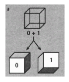
In the August 2008 (page 66) issue of Scientific American, Monroe and Wineland attempted to provide a “picture” of the superposition with a figure of the “ambiguous” cube.


