4.24: AB2 Proton NMR Using Tensor Algebra

The purpose of this tutorial is to deviate from the usual matrix mechanics approach to the ABC proton nmr system in order to illustrate a related method of analysis which uses tensor algebra. For a discussion of the traditional approach visit http://www.users.csbsju.edu/~frioux/nmr/Speclab4.htm. This site also provides general information on the quantum mechanics of nmr spectroscopy.

Nuclear spin operators and identity:

\[ \begin{matrix} I_x = \frac{1}{2} \begin{pmatrix} 0 & 1 \\ 1 & 0 \end{pmatrix} & I_y = \frac{1}{2} \begin{pmatrix} 0 & -i \\ i & 0 \end{pmatrix} & I_z = \frac{1}{2} \begin{pmatrix} 1 & 0 \\ 0 & -1 \end{pmatrix} & I = \begin{pmatrix} 1 & 0 \\ 0 & 1 \end{pmatrix} \end{matrix} \nonumber \]

The following experimentally determined chemical shifts and coupling constant (all in Hz) are for the AB₂ proton system 1,1,2-trichloroethane at 60 MHz.

\[ \begin{matrix} \text{Chemical shifts:} & \nu_A = 345.6 & \nu_B = 237.6 & Jab = 6.1 \end{matrix} \nonumber \]

Hamiltonian representing the interaction of nuclear spins with the external magnetic field in tensor format:

\[ \widehat{H}_{mag} = - \nu_A \hat{I}_z^A - \nu_B \hat{I}_z^B - \nu_C \hat{I}_z^C = \nu_A \hat{I}_z^A \otimes \hat{I} \otimes \hat{I} + \hat{I} \otimes \left( - \nu_B \hat{I}_z^B \right) \otimes \hat{I} + \hat{I} \otimes \hat{I} \otimes \left( - \nu_B \hat{I}_z^B \right) \nonumber \]

where, for example,

\[ \nu_A = g_n \beta_n B_z (1 - \sigma_A) \nonumber \]

Implementing the operator using Mathcad's command for the tensor product, kronecker, is as follows.

\[ H_{mag} = - \nu_A \text{kronecker} \left( I_z,~ \text{kronecker(I, I)} \right) - \nu_B \text{kronecker} (I,~ \text{kronecker} (I_z,~I)) - \nu_B \text{kronecker}(I,~ \text{kronecker}(I,~I_z)) \nonumber \]

Hamiltonian representing the interaction of nuclear spins with each other in tensor format:

\[ \begin{matrix} \widehat{H}_{spin} = J_{AB} \left( \hat{I}_x^A \otimes \hat{I}_x^B \otimes \hat{I} + \hat{I}_y^A \otimes \hat{I}_y^B \otimes \hat{I} + \hat{I}_z^A \otimes \hat{I}_z^B \otimes \hat{I} \right) \\ + J_{AB} \left( \hat{I}_x^A \otimes \hat{I} \otimes \hat{I}_x^B + \hat{I}_y^A \otimes \hat{I} \otimes \hat{I}_y^B + \hat{I}_z^A \otimes \hat{I} \otimes \hat{I}_z^B \right) \end{matrix} \nonumber \]

Implementation of the operator in the Mathcad programming environment:

\[ H_{spin} = \begin{matrix} Jab \left( \text{kronecker} (I_x,~ \text{kronecker} (I_x,~I)) \text{kronecker}(I_y,~ \text{kronecker}(I_y,~I)) + \text{kronecker}(I_z,~ \text{kronecker} (I_z,~I)) \right) ... \\ + \begin{bmatrix} Jab \left( \text{kronecker} (I_x,~ \text{kronecker}(I,~I_x)) + \text{kronecker} (I_y,~ \text{kronecker} (I,~I_y)) + \text{kronecker} (I_z,~ \text{kronecker}(I,~I_z)) \right) \end{bmatrix} \end{matrix} \nonumber \]

The total Hamiltonian spin operator is now calculated and displayed.

\[ H = H_{mag} + H_{spin} \nonumber \]

The indexing of the matrix elements of the Hamiltonial spin operator is discussed in the Appendix.

i = 1 .. 8

\[ H = \begin{pmatrix} -407.35 & 0 & 0 & 0 & 0 & 0 & 0 & 0 \\ 0 & -172.8 & 0 & 0 & 3.05 & 0 & 0 & 0 \\ 0 & 0 & -172.8 & 0 & 3.05 & 0 & 0 & 0 \\ 0 & 3.05 & 3.05 & 0 & -67.85 & 0 & 0 & 0 \\ 0 & 0 & 0 & 3.05 & 0 & 172.8 & 0 & 0 \\ 0 & 0 & 0 & 3.5 & 0 & 234.13 & 0.75 & 0 \\ 0 & 0 & 0 & 3.05 & 0 & 0 & 172.8 & 0 \\ 0 & 0 & 0 & 0 & 0 & 0 & 0 & 413.45 \end{pmatrix} \nonumber \]

Calculate and display the energy eigenvalues and associated eigenvectors of the Hamiltonian.

\[ \begin{matrix} E = \text{sort(eigenvals(H))} & C^{<i>} = \text{eigenvec}(H,~E_i ) \end{matrix} \nonumber \]

\[ \text{augment} \left( E,~C^T \right)^T = \begin{matrix} \begin{pmatrix} -407.35 & -172.977 & -172.8 & -67.673 & 61.583 & 172.8 & 172.967 & 413.45 \\ 1 & 0 & 0 & 0 & 0 & 0 & 0 & 0 \\ 0 & 0.707 & -0.707 & 0.029 & 0 & 0 & 0 & 0 \\ 0 & 0.707 & 0.707 & 0.029 & 0 & 0 & 0 & 0 \\ 0 & 0 & 0 & 0 & 0.999 & 0 & 0.039 & 0 \\ 0 & -0.041 & 0 & 0.999 & 0 & 0 & 0 & 0 \\ 0 & 0 & 0 & 0 & -0.027 & -0.707 & 0.707 & 0 \\ 0 & 0 & 0 & 0 & -0.027 & 0.707 & 0.707 & 0 \\ 0 & 0 & 0 & 0 & 0 & 0 & 0 & 1 \end{pmatrix} \begin{array} \\ \alpha \alpha \alpha \alpha \\ \alpha \alpha \beta \\ \alpha \beta \alpha \\ \alpha \beta \beta \\ \beta \alpha \alpha \\ \beta \alpha \beta \\ \beta \beta \alpha \\ \beta \beta \beta \end{array} \end{matrix} \nonumber \]

Notice that the ground state |ααα> and the highest excited state |βββ> are pure states. The other six states are strictly speaking superpositions.

The nmr selection rule is that only one nuclear spin can flip during a transition. Therefore, the transition probability matrix for the ABC spin system is:

\[ T = \begin{matrix} \begin{array} \alpha \alpha \alpha \alpha & \alpha \alpha \beta & \alpha \beta \alpha & \alpha \beta \beta & \beta \alpha \alpha & \beta \alpha \beta & \beta \beta \alpha & \beta \beta \beta \end{array} \\ \begin{pmatrix} 0 & 1.00 & 1.00 & 0 & 1.00 & 0 & 0 & 0 \\ 1.00 & 0 & 0 & 1.00 & 0 & 1.00 & 0 & 0 \\ 1.00 & 0 & 0 & 1.00 & 0 & 0 & 1.00 & 0 \\ 0 & 1.00 & 1.00 & 0 & 0 & 0 & 0 & 1.00 \\ 1.00 & 0 & 0 & 0 & 0 & 1.00 & 1.00 & 0 \\ 0 & 1.00 & 0 & 0 & 1.00 & 0 & 0 & 1.00 \\ 0 & 0 & 1.00 & 0 & 1.00 & 0 & 0 & 1.00 \\ 0 & 0 & 0 & 1.00 & 0 & 1.00 & 1.00 & 0 \end{pmatrix} \begin{array} \alpha \alpha \alpha \alpha \\ \alpha \alpha \beta \\ \alpha \beta \alpha \\ \alpha \beta \beta \\ \beta \alpha \alpha \\ \beta \alpha \beta \\ \beta \beta \alpha \\ \beta \beta \beta \end{array} \end{matrix} \nonumber \]

Calculate the intensities and frequencies of the allowed transitions.

\[ \begin{matrix} i = 1 .. 8 & j = 1 .. 8 & I_{i,~j} = \left[ C^{<i>} \left( TC^{<j>} \right) \right]^2 & V_{i,~j} = \text{ if}(I_{i,~j} . .001,~ \left| E_i - E_j \right|,~0) \end{matrix} \nonumber \]

Intensity matrix:

\[ i = \begin{pmatrix} 0 & 1.88 & 0 & 1.12 & 0 & 0 & 0 & 0 \\ 1.88 & 0 & 0 & 0 & 1.89 & 0 & 0.99 & 0 \\ 0 & 0 & 0 & 0 & 0 & 1 & 0 & 0 \\ 1.12 & 0 & 0 & 0 & 0 & 0 & 2.12 & 0 \\ 0 & 1.89 & 0 & 0 & 0 & 0 & 0 & 0.89 \\ 0 & 0 & 1 & 0 & 0 & 0 & 0 & 0 \\ 0 & 0.99 & 0 & 2.12 & 0 & 0 & 0 & 2.11 \\ 0 & 0 & 0 & 0 & 0.89 & 0 & 2.11 & 0 \end{pmatrix} \nonumber \]

Frequency matrix:

\[ \text{V} = \begin{pmatrix} 0 & 234.37 & 234.55 & 339.68 & 468.93 & 580.15 & 580.32 & 820.8 \\ 234.37 & 0 & 0.18 & 105.3 & 234.56 & 345.78 & 345.94 & 586.43 \\ 234.55 & 0.18 & 0 & 105.13 & 234.38 & 345.6 & 345.77 & 586.25 \\ 339.68 & 105.3 & 105.13 & 0 & 129.26 & 240.47 & 240.64 & 481.12 \\ 468.93 & 234.56 & 234.38 & 129.26 & 0 & 111.22 & 111.38 & 351.87 \\ 580.15 & 345.78 & 345.6 & 240.47 & 111.22 & 0 & 0.17 & 240.65 \\ 580.32 & 345.94 & 345.77 & 240.64 & 111.38 & 0.17 & 0 & 240.48 \\ 820.8 & 586.43 & 586.25 & 481.12 & 351.87 & 240.65 & 240.48 & 0 \end{pmatrix} \nonumber \]

Display the calculated vinyl acetate nmr spectrum:

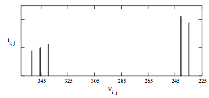
The calculated spectrum compares favorably with experimental spectrum, indicating that the spin Hamiltonian used adequately represents the magnetic interaction of the protons in 1,1,2-trichloroethane at 60 MHz.

Appendix

The tensor product of three spinors is shown below.

\[ \begin{pmatrix} a \\ b \end{pmatrix} \otimes \begin{pmatrix} c \\ d \end{pmatrix} \otimes \begin{pmatrix} e \\ f \end{pmatrix} = \begin{pmatrix} a \\ b \end{pmatrix} \otimes \begin{pmatrix} ce \\ cf \\ de \\ df \end{pmatrix} = \begin{pmatrix} ace \\ acf \\ ade \\ adf \\ bce \\ bcf \\ bde \\ bdf \end{pmatrix} \nonumber \]

Mathcad does not have a command for this type of vector tensor product, so it is necessary to develop a way of implementing it using kronecker, which requires square matrices. For this reason the spin vector is stored in the left column of a 2x2 matrix by augmenting the spin vector with the null vector. After all the matrix tensor products have been carried out using kronecker the final spin vector resides in the left column of the final square matrix. Next the submatrix cammand is used to save this column, discarding the rest of the matrix.

\[ \begin{matrix} \text{Spin-up in the z-direction:} & \alpha = \begin{pmatrix} 1 \\ 0 \end{pmatrix} & \text{Spin-down in the z-direction:} & \beta = \begin{pmatrix} 0 \\ 1 \end{pmatrix} & \text{Null vector:} & N = \begin{pmatrix} 0 \\ 0 \end{pmatrix} \end{matrix} \nonumber \]

The eight possible spin states of a three-proton system are calculated as shown below.

\[ \Psi \text{(a, b, c) = submatrix(kronecker(augment(a, N), kronecker(augment(b, N), augment(c, N))), 1, 8, 1, 1)} \nonumber \]

\[ \begin{matrix} \Psi ( \alpha, \alpha, \alpha )^T = \begin{pmatrix} 1 & 0 & 0 & 0 & 0 & 0 & 0 & 0 \end{pmatrix} & \Psi ( \alpha, \alpha, \beta )^T = \begin{pmatrix} 0 & 1 & 0 & 0 & 0 & 0 & 0 & 0 \end{pmatrix} \\ \Psi ( \alpha, \beta, \alpha )^T = \begin{pmatrix} 0 & 0 & 1 & 0 & 0 & 0 & 0 & 0 \end{pmatrix} & \Psi ( \alpha, \beta, \beta )^T = \begin{pmatrix} 0 & 0 & 0 & 1 & 0 & 0 & 0 & 0 \end{pmatrix} \\ \Psi ( \beta, \alpha, \alpha )^T = \begin{pmatrix} 0 & 0 & 0 & 0 & 1 & 0 & 0 & 0 \end{pmatrix} & \Psi ( \beta, \alpha, \beta )^T = \begin{pmatrix} 0 & 0 & 0 & 0 & 1 & 0 & 0 & 0 \end{pmatrix} \\ \Psi ( \beta, \beta, \alpha )^T = \begin{pmatrix} 0 & 0 & 0 & 0 & 0 & 0 & 1 & 0 \end{pmatrix} & \Psi ( \beta, \beta, \beta )^T = \begin{pmatrix} 0 & 0 & 0 & 0 & 0 & 0 & 0 & 1 \end{pmatrix} \end{matrix} \nonumber \]

Thus the indexing in Hamiltonian matrix is: |ααα>, |ααβ>, |αβα>, |αββ>, |βαα>, |βαβ>, |ββα>, |βββ>.