2.12: Hydrogen-Like Calculations with Variable Lepton Mass

Under normal circumstances the the hydrogen atom consists of a proton and an electron. However, electrons are leptons and there are two other leptons which could temporarily replace the electron in the hydrogen atom. The other leptons are the muon and tauon, and their relevant properties, along with those of the electron, are given in the following table. The following calculations are carried out in atomic units (me = e = h/2π = 1) and are valid for any one‐lepton atom or ion.

\[ \begin{pmatrix} \text{Property} & e & \mu & \tau \\ \frac{ \text{Mass}}{m_e} & 1 & 206.8 & 3491 \\ \frac{ \text{EffectiveMass}}{m_e} & 1 & 185.86 & 1203 \\ \frac{ \text{LifeTime}}{s} & \text{Stable} & 2.2 (10)^{-6} & 3.0 (10)^{-13} \end{pmatrix} \nonumber \]

Coordinate‐space calculations:

Energy operator:

\[ H = - \frac{1}{2 \mu} \frac{d^2}{dx^2} \blacksquare - \frac{1}{x} \blacksquare \nonumber \]

Trial ground state wave function:

\[ \begin{matrix} \Psi (x,~ \mu) = 2 \mu^{ \frac{3}{2}} x \text{exp} ( - \mu,~x) & \int_0^{ \infty} \Psi (x,~ \mu)^2 \text{dx assume}, \mu > 0 \rightarrow 1 \end{matrix} \nonumber \]

Demonstrate that the wave function is an eigenfunction of the total energy operator, but not of the kinetic and potential energy operators individually:

\[ \begin{matrix} - \frac{1}{2 \mu} \frac{d^2}{dx^2} \Psi (x,~ \mu) - \frac{1}{x} \Psi (x,~ \mu) = E \Psi (x,~ \mu ) \text{solve, E} \rightarrow \frac{-1}{2} \mu \\ \frac{- \frac{1}{2 \mu} \frac{d^2}{dx^2} \Psi (x,~ \mu )}{\Psi (x, ~ \mu )} \text{simplify} \rightarrow \frac{-1}{2} \frac{(-2) + \mu x}{x} ~ \frac{- \frac{1}{x} \Psi (x, ~ \mu)}{ \Psi (x, ~ \mu)} \rightarrow \frac{-1}{x} \end{matrix} \nonumber \]

Calculate <T>:

\[ \int_0^{ \infty} \Psi (x,~ \mu ) - \frac{1}{2 \mu} \frac{d^2}{dx^2} \Psi (x,~ \mu ) \text{dx assume, } \mu > 0 \rightarrow \frac{1}{2} \mu \nonumber \]

Calculate <R>:

\[ \int_0 ^{ \infty} \Psi (x,~ \mu) \frac{-1}{x} \Psi (x,~ \mu) \text{ dx assume, } \mu >0 \rightarrow - \mu \nonumber \]

Is the virial theorem satisfied? Yes.

\[ <E> = \frac{<V>}{2} = -<T> = \frac{ \mu}{2} \nonumber \]

Calculate the classical turning point:

\[ \frac{- \mu}{2} = \frac{-1}{x} \text{ solve, x} \rightarrow \frac{2}{ \mu} \nonumber \]

Calculate the probability that tunneling is occurring:

\[ \int_{ \frac{2}{ \mu}}^{ \infty} \Psi (x,~ \mu)^2 \text{ dx assume, } \mu > 0 \rightarrow 13 e^{-4} = 0.238 \nonumber \]

Calculate <x>:

\[ \int_0 ^{ \infty} x \Psi (x,~ \mu)^2 \text{ dx assume, } \mu > 0 \rightarrow \frac{3}{2 \mu} \nonumber \]

Calculate <x²>:

\[ \int_0^{ \infty} x^2 \Psi (x,~ \mu )^2 \text{ dx assume, } \mu > 0 \rightarrow \frac{3}{ \mu^2} \nonumber \]

Calculate the most probable position:

\[ \frac{d}{dx} \Psi (x,~ \mu) = 0 \text{solve, x} \rightarrow \frac{1}{ \mu} \nonumber \]

Calculate the electron density at the most probable position:

\[ \begin{matrix} \Psi \left( \frac{1}{ \mu},~ \mu \right)^2 \rightarrow 4 \mu \left( e^{-1} \right)^2 & 0.541 \mu \end{matrix} \nonumber \]

Calculate the probability the electron is beyond the most probable position:

\[ \int_{ \frac{1}{ \mu}}^{ \infty} \text{ dx assume, } \mu > 0 \rightarrow 5 e^{-2} = 0.677 \nonumber \]

Calculate

:

\[ \int_0^{ \infty} \Psi (x,~ \mu) \frac{1}{i} \frac{d}{dx} \Psi (x,~ \mu) \text{dx assume, } \mu > 0 \rightarrow \nonumber \]

Calculate <p²>:

\[ \int_0^{ \infty} \Psi (x,~ \mu) - \frac{d^2}{dx^2} \Psi (x,~ \mu) \text{ dx assume, } \mu >0 \rightarrow \mu^2 \nonumber \]

Calculate the position-momentum commutator:

\[ \frac{x \frac{1}{i} \frac{d}{dx} \Psi (x,~ \mu) - \frac{1}{i} \frac{d}{dx} (x \Psi (x,~ \mu))}{ \Psi (x, \mu )} \text{simplify} \rightarrow i \nonumber \]

Momentum-space calculations:

Generate the momentum wave function by Fourier transform of the coordinate-space wave function:

\[ \Phi (p,~ \mu) = \int_0^{ \infty} \frac{ \text{exp} (-i px)}{ \sqrt{2 \pi}} \Psi (x,~ \mu) \text{ dx assume, } \mu > 0 \rightarrow 2^{ \frac{1}{2}} \frac{}{} \nonumber \]

Calculate <T>:

\[ \int_{- \infty}^{ \infty} \overline{ \Phi (p,~ \mu)} \frac{p^2}{2 \mu} \Phi (p,~ \mu ) \text{ dp assume, } \mu > 0 \rightarrow \frac{1}{2} \mu \nonumber \]

Calculate <x>:

\[ \begin{array}{c|c} \int_{ - \infty}^{ \infty} \overline{ \Phi (p,~u)} i \frac{d}{dp} \Phi (p,~u) dp & _{ \text{simplify}}^{ \text{assume, } \mu >0} \rightarrow \frac{3}{ \mu} \end{array} \nonumber \]

Calculate <x²>:

\[ \begin{array}{c|c} \int_{ - \infty}^{ \infty} \overline{ \Phi (p,~u)} - \frac{d}{dp} \Phi (p,~u) dp & _{ \text{simplify}}^{ \text{assume, } \mu >0} \rightarrow \frac{3}{ \mu^2} \end{array} \nonumber \]

Calculate

:

\[ \int_{ - \infty}^{ \infty} \overline{ \Phi (p,~u)} p \Phi (p,~ \mu ) \text{ dp assume, } \mu > 0 \rightarrow 0 \nonumber \]

Calculate <p²>:

\[ \int_{ - \infty}^{ \infty} \overline{ \Phi (p,~u)} p^2 \Phi (p,~ \mu ) \text{ dp assume, } \mu > 0 \rightarrow \mu^2 \nonumber \]

Calculate Δx:

\[ \sqrt{ \frac{3}{ \mu^2} - \left( \frac{3}{2 \mu} \right)^2} = \frac{ \sqrt{2}}{2 \mu} \nonumber \]

Calculate Δp:

\[ \sqrt{ \mu^2} = \mu \nonumber \]

Calculate ΔxΔp:

\[ \frac{ \sqrt{3}}{2} = 0.866 \nonumber \]

The uncertainty principle is obeyed because the result is greater than 0.5.

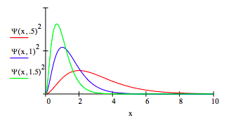
Spatial distribution as a function of μ:

Momentum distribution as a function of μ:

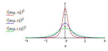
The spatial and momentum distributions provide a graphical illustration of the uncertainty principle.