2.9: Extracting Atomic and Molecular Parameters from the deBroglie-Bohn Model for the Atom
- Page ID
- 154880
\( \newcommand{\vecs}[1]{\overset { \scriptstyle \rightharpoonup} {\mathbf{#1}} } \)
\( \newcommand{\vecd}[1]{\overset{-\!-\!\rightharpoonup}{\vphantom{a}\smash {#1}}} \)
\( \newcommand{\id}{\mathrm{id}}\) \( \newcommand{\Span}{\mathrm{span}}\)
( \newcommand{\kernel}{\mathrm{null}\,}\) \( \newcommand{\range}{\mathrm{range}\,}\)
\( \newcommand{\RealPart}{\mathrm{Re}}\) \( \newcommand{\ImaginaryPart}{\mathrm{Im}}\)
\( \newcommand{\Argument}{\mathrm{Arg}}\) \( \newcommand{\norm}[1]{\| #1 \|}\)
\( \newcommand{\inner}[2]{\langle #1, #2 \rangle}\)
\( \newcommand{\Span}{\mathrm{span}}\)
\( \newcommand{\id}{\mathrm{id}}\)
\( \newcommand{\Span}{\mathrm{span}}\)
\( \newcommand{\kernel}{\mathrm{null}\,}\)
\( \newcommand{\range}{\mathrm{range}\,}\)
\( \newcommand{\RealPart}{\mathrm{Re}}\)
\( \newcommand{\ImaginaryPart}{\mathrm{Im}}\)
\( \newcommand{\Argument}{\mathrm{Arg}}\)
\( \newcommand{\norm}[1]{\| #1 \|}\)
\( \newcommand{\inner}[2]{\langle #1, #2 \rangle}\)
\( \newcommand{\Span}{\mathrm{span}}\) \( \newcommand{\AA}{\unicode[.8,0]{x212B}}\)
\( \newcommand{\vectorA}[1]{\vec{#1}} % arrow\)
\( \newcommand{\vectorAt}[1]{\vec{\text{#1}}} % arrow\)
\( \newcommand{\vectorB}[1]{\overset { \scriptstyle \rightharpoonup} {\mathbf{#1}} } \)
\( \newcommand{\vectorC}[1]{\textbf{#1}} \)
\( \newcommand{\vectorD}[1]{\overrightarrow{#1}} \)
\( \newcommand{\vectorDt}[1]{\overrightarrow{\text{#1}}} \)
\( \newcommand{\vectE}[1]{\overset{-\!-\!\rightharpoonup}{\vphantom{a}\smash{\mathbf {#1}}}} \)
\( \newcommand{\vecs}[1]{\overset { \scriptstyle \rightharpoonup} {\mathbf{#1}} } \)
\( \newcommand{\vecd}[1]{\overset{-\!-\!\rightharpoonup}{\vphantom{a}\smash {#1}}} \)
\(\newcommand{\avec}{\mathbf a}\) \(\newcommand{\bvec}{\mathbf b}\) \(\newcommand{\cvec}{\mathbf c}\) \(\newcommand{\dvec}{\mathbf d}\) \(\newcommand{\dtil}{\widetilde{\mathbf d}}\) \(\newcommand{\evec}{\mathbf e}\) \(\newcommand{\fvec}{\mathbf f}\) \(\newcommand{\nvec}{\mathbf n}\) \(\newcommand{\pvec}{\mathbf p}\) \(\newcommand{\qvec}{\mathbf q}\) \(\newcommand{\svec}{\mathbf s}\) \(\newcommand{\tvec}{\mathbf t}\) \(\newcommand{\uvec}{\mathbf u}\) \(\newcommand{\vvec}{\mathbf v}\) \(\newcommand{\wvec}{\mathbf w}\) \(\newcommand{\xvec}{\mathbf x}\) \(\newcommand{\yvec}{\mathbf y}\) \(\newcommand{\zvec}{\mathbf z}\) \(\newcommand{\rvec}{\mathbf r}\) \(\newcommand{\mvec}{\mathbf m}\) \(\newcommand{\zerovec}{\mathbf 0}\) \(\newcommand{\onevec}{\mathbf 1}\) \(\newcommand{\real}{\mathbb R}\) \(\newcommand{\twovec}[2]{\left[\begin{array}{r}#1 \\ #2 \end{array}\right]}\) \(\newcommand{\ctwovec}[2]{\left[\begin{array}{c}#1 \\ #2 \end{array}\right]}\) \(\newcommand{\threevec}[3]{\left[\begin{array}{r}#1 \\ #2 \\ #3 \end{array}\right]}\) \(\newcommand{\cthreevec}[3]{\left[\begin{array}{c}#1 \\ #2 \\ #3 \end{array}\right]}\) \(\newcommand{\fourvec}[4]{\left[\begin{array}{r}#1 \\ #2 \\ #3 \\ #4 \end{array}\right]}\) \(\newcommand{\cfourvec}[4]{\left[\begin{array}{c}#1 \\ #2 \\ #3 \\ #4 \end{array}\right]}\) \(\newcommand{\fivevec}[5]{\left[\begin{array}{r}#1 \\ #2 \\ #3 \\ #4 \\ #5 \\ \end{array}\right]}\) \(\newcommand{\cfivevec}[5]{\left[\begin{array}{c}#1 \\ #2 \\ #3 \\ #4 \\ #5 \\ \end{array}\right]}\) \(\newcommand{\mattwo}[4]{\left[\begin{array}{rr}#1 \amp #2 \\ #3 \amp #4 \\ \end{array}\right]}\) \(\newcommand{\laspan}[1]{\text{Span}\{#1\}}\) \(\newcommand{\bcal}{\cal B}\) \(\newcommand{\ccal}{\cal C}\) \(\newcommand{\scal}{\cal S}\) \(\newcommand{\wcal}{\cal W}\) \(\newcommand{\ecal}{\cal E}\) \(\newcommand{\coords}[2]{\left\{#1\right\}_{#2}}\) \(\newcommand{\gray}[1]{\color{gray}{#1}}\) \(\newcommand{\lgray}[1]{\color{lightgray}{#1}}\) \(\newcommand{\rank}{\operatorname{rank}}\) \(\newcommand{\row}{\text{Row}}\) \(\newcommand{\col}{\text{Col}}\) \(\renewcommand{\row}{\text{Row}}\) \(\newcommand{\nul}{\text{Nul}}\) \(\newcommand{\var}{\text{Var}}\) \(\newcommand{\corr}{\text{corr}}\) \(\newcommand{\len}[1]{\left|#1\right|}\) \(\newcommand{\bbar}{\overline{\bvec}}\) \(\newcommand{\bhat}{\widehat{\bvec}}\) \(\newcommand{\bperp}{\bvec^\perp}\) \(\newcommand{\xhat}{\widehat{\xvec}}\) \(\newcommand{\vhat}{\widehat{\vvec}}\) \(\newcommand{\uhat}{\widehat{\uvec}}\) \(\newcommand{\what}{\widehat{\wvec}}\) \(\newcommand{\Sighat}{\widehat{\Sigma}}\) \(\newcommand{\lt}{<}\) \(\newcommand{\gt}{>}\) \(\newcommand{\amp}{&}\) \(\definecolor{fillinmathshade}{gray}{0.9}\)The 1913 Bohr model of the hydrogen atom was replaced by Schrödingerʹs wave mechanical model in 1926. However, Bohrʹs model is still profitably taught today because of its conceptual and mathematical simplicity, and because it introduced a number of key quantum mechanical ideas such as the quantum number, quantization of observable properties, quantum jump and stationary state. In addition it provided realistic values for such parameters as atomic and molecular size, electron ionization energy, and molecular bond energy.
In his ʺplanetaryʺ model of the hydrogen atom Bohr began with a Newtonian analysis of the electron executing a circular orbit of radius R about a stationary nucleus, and then arbitrarily quantized the electronʹs angular momentum. Finally, by fiat he declared that the electron was in a non‐radiating stationary state because an orbiting (accelerating) charge radiates energy and will collapse into the oppositely charge nucleus.
In 1924 de Broglie postulated wave‐particle duality for the electron and other massive particles, thereby providing the opportunity to remove some of the arbitrariness from Bohrʹs model. For example, an electron possessing wave properties is subject to constructive and destructive interference. As will be shown this leads naturally to quantization of electron momentum and kinetic energy, and consequently to a stable ground state for the hydrogen atom.
The de Broglie‐Bohr model of the hydrogen atom presented here treats the electron as a particle on a ring with wave‐like properties. The key equation is wave‐particle duality as expressed by the de Broglie equation. The particle concept momentum and the wave concept λ are joined in a reciprocal relationship mediated by the ubiquitous Planckʹs constant.
\[ p = \frac{h}{ \lambda} \nonumber \]
This equation will be used with the Bohr model of the hydrogen atom to explain atomic stability and to generate estimates of atomic size and electron binding energy in the atom.
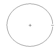
In the de Broglie version of the Bohr hydrogen atom we say that the electron occupies a ring of radius R. It is not orbiting the nucleus, it is behaving as a stationary wave. In order to avoid self‐interference the following wavelength restriction must be obeyed for the ground state of the hydrogen atom.
\[ \lambda = 2 \pi R \nonumber \]
When combined with the de Broglie equation it reveals the following restriction on the electron's particle property, linear momentum.
\[ p = \frac{h}{2 \pi R} \nonumber \]
This means that there is also a restriction on the electron's kinetic energy. Use of this equation in the classical expression for kinetic energy yields the quantum mechanical kinetic energy or more accurately electron confinement energy.
\[ T = \frac{p^2}{2m} = \frac{h^2}{8 \pi^2 m R^2} = \frac{1}{2R^2} \nonumber \]
In this equation we have moved from the classical definition of kinetic energy to the quantum mechanical version expressed on the right in atomic units.
\[ \frac{h}{2 \pi} = m = e = 4 \pi \varepsilon_0 = 1 \nonumber \]
The electrostatic potential energy retains its classical definition in quantum mechanics.
\[ V = \frac{-e^2}{4 \pi \varepsilon_0 R} = \frac{-1}{R} \nonumber \]
The total electron energy, \( E_H (R) = T(R) + V(R)\), is now minimized with respect to the ring or orbit radius, the only variational parameter in the model. The total energy, and kinetic and potential energy, are also displayed as a function of ring radius.
\[ \begin{matrix} R = .5 & E_H (R) = \frac{1}{2R^2} - \frac{1}{R} & R = \text{Minimize} \left( E_H,~R \right) & R = 1.000 & E_H (R) = -0.500 \end{matrix} \nonumber \]
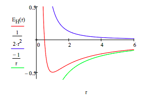
From this simple model we learn that it is the wave nature of the electron that explains atomic stability. The electronʹs ring does not collapse into the nucleus because kinetic (confinement) energy goes to positive infinity (~R‐2) faster than potential energy goes to negative infinity (~‐R‐1). This is seen very clearly in the graph. The ground state is due to the sharp increase in kinetic energy as the ring radius decreases. This is a quantum effect, a consequence of de Broglieʹs hypothesis that electrons have wave‐like properties. As Klaus Ruedenberg has written, ʺThere are no ground states in classical mechanics.ʺ
The minimization process above the figure provides the ground state ring radius and electron energy in atomic units, a0 and Eh, respectively. R = 1 a0 = 52.9 pm gives us the benchmark for atomic size. Tables of atomic and ionic radii carry entries ranging from approximately half this value to roughly five or six times it. The ground state (binding) energy, E = ‐0.5 Eh = ‐13.6 eV = ‐1312 kJ/mol, is the negative of the ionization energy. This value serves as a benchmark for how tightly electrons are held in atoms and molecules.
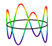
A more comprehensive treatment of the Bohr atom utilizing the restriction that an integral number of wavelengths must fit within the ring, nλ = 2πR , where n = 1, 2, 3, ... reveals a manifold of allowed energy states (‐0.5 Eh/n2) and the basis for Bohrʹs concept of the quantum jump which ʺexplainedʺ the hydrogen atom emission spectrum. Here for example is the n = 4 Bohr atom excited state.
Rudimentary estimates of some molecular parameters, the most important being bond energy and bond length, can be obtained using the following Bohr model for H2. The distance between the protons is D, the electron ring radius is R, and the bond axis is perpendicular to the plane of the ring.
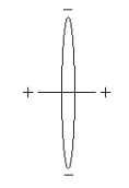
There are eight contributions to the total molecular energy based on this model: electron kinetic energy (2), electron‐proton potential energy (4), proton‐proton potential energy (1) and electron‐electron potential energy (1).
\[ E_{H2} (R,~D) = \frac{1}{R^2} = \frac{4}{ \sqrt{R^2 + \left( \frac{D}{2} \right)^2}} + \frac{1}{D} + \frac{1}{2R} \nonumber \]
Minimization of the energy with respect to ring radius and proton‐proton distance yields the following results.
\[ \begin{matrix} D = 2 & \begin{pmatrix} R \\ D \end{pmatrix} = \text{Minimize} \left( E_{H2},~R,~D \right) & \begin{pmatrix} R \\ D \end{pmatrix} = \begin{pmatrix} 0.953 \\ 1.101 \end{pmatrix} & E_{H2} (R,~D) = -1.100 \end{matrix} \nonumber \]
The H‐H bond energy is the key parameter provided by this analysis. We see that it predicts a stable molecule and that the energy released on the formation of H2 is 0.1 Eh or 263 kJ/mol, compared with the experimental value of 458 kJ/mol. The model predicts a H‐H bond length of 58 pm (D.52.9 pm), compared to the literature value of 74 pm. These results are acceptable given the primitive character of the model.
\[ H + H = H_2 \nonumber \]
\[ \begin{matrix} \Delta E_{bond} = E_{H2} (R,~D) - 2 E_H (1) & \Delta E_{bond} = -0.100 \end{matrix} \nonumber \]
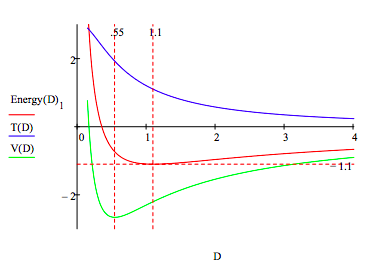
In addition to these estimates of molecular parameters, the model clearly shows that molecular stability depends on a balancing act between electron‐proton attraction and the ʺrepulsiveʺ character of electron kinetic energy. Just as in the atomic case, it is the 1/R2 dependence of kinetic (confinement) energy on ring radius that prevents molecular collapse under electron‐proton attraction. As the energy profile provided in the Appendix shows, the immediate cause of the molecular ground state is a rise in kinetic energy. Potential energy is still declining at this point and does not begin to rise until 0.55 a0, well after the ground state is reached at 1.10 a0.
Although the model is a relic from the early days of quantum theory it still has pedagogical value. Its mathematical simplicity clearly reveals the importance of the wave nature of matter, the foundational concept of quantum theory.
Two relatively recent appraisals of Bohrʹs models of atomic and molecular structure have been appeared in Physics Today:
- ʺNiels Bohr between physics and chemistry,ʺ by Helge Kragh, May 2013, 36‐41.
- ʺBohrʹs molecular model, a century later,ʺ by Anatoly Svidzinsky, Marlan Scully, and Dudley Herschbach, January 2014, 33‐39.
Appendix
\[ \begin{matrix} R = .1 & \text{Energy} = -1 & \text{Given} & \text{Energy} = E_{H2} (R,~D) & \frac{d}{dR} E_{H2} (R,~D) = 0 & \text{Energy(D) = Find(R, Energy)} \end{matrix} \nonumber \]
\[ \begin{matrix} D = .15,~.16 ..4 & T(D) = \frac{1}{ \left( \text{Energy(D)}_0 \right)^2} & V(D) = - \frac{4}{ \sqrt{ \left( \text{Energy(D)}_0 \right)^2 + \left( \frac{D}{2} \right)^2 }} + \frac{1}{D} + \frac{1}{2 \text{Energy (D)}_0} \end{matrix} \nonumber \]
