
1.72: Superposition vs. Mixture
- Page ID
- 156462

\( \newcommand{\vecs}[1]{\overset { \scriptstyle \rightharpoonup} {\mathbf{#1}} } \)
\( \newcommand{\vecd}[1]{\overset{-\!-\!\rightharpoonup}{\vphantom{a}\smash {#1}}} \)
\( \newcommand{\id}{\mathrm{id}}\) \( \newcommand{\Span}{\mathrm{span}}\)
( \newcommand{\kernel}{\mathrm{null}\,}\) \( \newcommand{\range}{\mathrm{range}\,}\)
\( \newcommand{\RealPart}{\mathrm{Re}}\) \( \newcommand{\ImaginaryPart}{\mathrm{Im}}\)
\( \newcommand{\Argument}{\mathrm{Arg}}\) \( \newcommand{\norm}[1]{\| #1 \|}\)
\( \newcommand{\inner}[2]{\langle #1, #2 \rangle}\)
\( \newcommand{\Span}{\mathrm{span}}\)
\( \newcommand{\id}{\mathrm{id}}\)
\( \newcommand{\Span}{\mathrm{span}}\)
\( \newcommand{\kernel}{\mathrm{null}\,}\)
\( \newcommand{\range}{\mathrm{range}\,}\)
\( \newcommand{\RealPart}{\mathrm{Re}}\)
\( \newcommand{\ImaginaryPart}{\mathrm{Im}}\)
\( \newcommand{\Argument}{\mathrm{Arg}}\)
\( \newcommand{\norm}[1]{\| #1 \|}\)
\( \newcommand{\inner}[2]{\langle #1, #2 \rangle}\)
\( \newcommand{\Span}{\mathrm{span}}\) \( \newcommand{\AA}{\unicode[.8,0]{x212B}}\)
\( \newcommand{\vectorA}[1]{\vec{#1}} % arrow\)
\( \newcommand{\vectorAt}[1]{\vec{\text{#1}}} % arrow\)
\( \newcommand{\vectorB}[1]{\overset { \scriptstyle \rightharpoonup} {\mathbf{#1}} } \)
\( \newcommand{\vectorC}[1]{\textbf{#1}} \)
\( \newcommand{\vectorD}[1]{\overrightarrow{#1}} \)
\( \newcommand{\vectorDt}[1]{\overrightarrow{\text{#1}}} \)
\( \newcommand{\vectE}[1]{\overset{-\!-\!\rightharpoonup}{\vphantom{a}\smash{\mathbf {#1}}}} \)
\( \newcommand{\vecs}[1]{\overset { \scriptstyle \rightharpoonup} {\mathbf{#1}} } \)
\( \newcommand{\vecd}[1]{\overset{-\!-\!\rightharpoonup}{\vphantom{a}\smash {#1}}} \)
\(\newcommand{\avec}{\mathbf a}\) \(\newcommand{\bvec}{\mathbf b}\) \(\newcommand{\cvec}{\mathbf c}\) \(\newcommand{\dvec}{\mathbf d}\) \(\newcommand{\dtil}{\widetilde{\mathbf d}}\) \(\newcommand{\evec}{\mathbf e}\) \(\newcommand{\fvec}{\mathbf f}\) \(\newcommand{\nvec}{\mathbf n}\) \(\newcommand{\pvec}{\mathbf p}\) \(\newcommand{\qvec}{\mathbf q}\) \(\newcommand{\svec}{\mathbf s}\) \(\newcommand{\tvec}{\mathbf t}\) \(\newcommand{\uvec}{\mathbf u}\) \(\newcommand{\vvec}{\mathbf v}\) \(\newcommand{\wvec}{\mathbf w}\) \(\newcommand{\xvec}{\mathbf x}\) \(\newcommand{\yvec}{\mathbf y}\) \(\newcommand{\zvec}{\mathbf z}\) \(\newcommand{\rvec}{\mathbf r}\) \(\newcommand{\mvec}{\mathbf m}\) \(\newcommand{\zerovec}{\mathbf 0}\) \(\newcommand{\onevec}{\mathbf 1}\) \(\newcommand{\real}{\mathbb R}\) \(\newcommand{\twovec}[2]{\left[\begin{array}{r}#1 \\ #2 \end{array}\right]}\) \(\newcommand{\ctwovec}[2]{\left[\begin{array}{c}#1 \\ #2 \end{array}\right]}\) \(\newcommand{\threevec}[3]{\left[\begin{array}{r}#1 \\ #2 \\ #3 \end{array}\right]}\) \(\newcommand{\cthreevec}[3]{\left[\begin{array}{c}#1 \\ #2 \\ #3 \end{array}\right]}\) \(\newcommand{\fourvec}[4]{\left[\begin{array}{r}#1 \\ #2 \\ #3 \\ #4 \end{array}\right]}\) \(\newcommand{\cfourvec}[4]{\left[\begin{array}{c}#1 \\ #2 \\ #3 \\ #4 \end{array}\right]}\) \(\newcommand{\fivevec}[5]{\left[\begin{array}{r}#1 \\ #2 \\ #3 \\ #4 \\ #5 \\ \end{array}\right]}\) \(\newcommand{\cfivevec}[5]{\left[\begin{array}{c}#1 \\ #2 \\ #3 \\ #4 \\ #5 \\ \end{array}\right]}\) \(\newcommand{\mattwo}[4]{\left[\begin{array}{rr}#1 \amp #2 \\ #3 \amp #4 \\ \end{array}\right]}\) \(\newcommand{\laspan}[1]{\text{Span}\{#1\}}\) \(\newcommand{\bcal}{\cal B}\) \(\newcommand{\ccal}{\cal C}\) \(\newcommand{\scal}{\cal S}\) \(\newcommand{\wcal}{\cal W}\) \(\newcommand{\ecal}{\cal E}\) \(\newcommand{\coords}[2]{\left\{#1\right\}_{#2}}\) \(\newcommand{\gray}[1]{\color{gray}{#1}}\) \(\newcommand{\lgray}[1]{\color{lightgray}{#1}}\) \(\newcommand{\rank}{\operatorname{rank}}\) \(\newcommand{\row}{\text{Row}}\) \(\newcommand{\col}{\text{Col}}\) \(\renewcommand{\row}{\text{Row}}\) \(\newcommand{\nul}{\text{Nul}}\) \(\newcommand{\var}{\text{Var}}\) \(\newcommand{\corr}{\text{corr}}\) \(\newcommand{\len}[1]{\left|#1\right|}\) \(\newcommand{\bbar}{\overline{\bvec}}\) \(\newcommand{\bhat}{\widehat{\bvec}}\) \(\newcommand{\bperp}{\bvec^\perp}\) \(\newcommand{\xhat}{\widehat{\xvec}}\) \(\newcommand{\vhat}{\widehat{\vvec}}\) \(\newcommand{\uhat}{\widehat{\uvec}}\) \(\newcommand{\what}{\widehat{\wvec}}\) \(\newcommand{\Sighat}{\widehat{\Sigma}}\) \(\newcommand{\lt}{<}\) \(\newcommand{\gt}{>}\) \(\newcommand{\amp}{&}\) \(\definecolor{fillinmathshade}{gray}{0.9}\)The Wigner function can be used to illustrate the difference between a superposition and a mixture. First consider the following linear superposition of Gaussian functions.
\[
\Psi(x) :=\exp \left[-(x-5)^{2}\right]+\exp \left[-(x+5)^{2}\right]
\nonumber \]
The Wigner distribution for this function is calculated and plotted below.
\[
\mathrm{W}(\mathrm{x}, \mathrm{p}) :=\int_{-\infty}^{\infty}\left[\exp \left[-\left(\mathrm{x}+\frac{\mathrm{s}}{2}-5\right)^{2}\right]+\exp \left[-\left(\mathrm{x}+\frac{\mathrm{s}}{2}+5\right)^{2}\right]\right] \cdot \exp (\mathrm{i} \cdot \mathrm{p} \cdot \mathrm{s}) \cdot\left[\exp \left[-\left(\mathrm{x}-\frac{\mathrm{s}}{2}-5\right)^{2}\right]+\exp \left[-\left(\mathrm{x}-\frac{\mathrm{s}}{2}+5\right)^{2}\right]\right] \mathrm{ds}
\nonumber \]
Integration yields:
\[
\mathrm{W}(\mathrm{x}, \mathrm{p}) :=\sqrt{2} \cdot \sqrt{\pi}\cdot\left(2 \cdot \exp \left(-2 \cdot \mathrm{x}^{2}-\frac{1}{2} \cdot \mathrm{p}^{2}\right) \cdot \cos (10 \cdot \mathrm{p})+\exp \left(-2 \cdot x^{2}+20 \cdot x-50-\frac{1}{2} \cdot p^{2}\right)+\exp \left(-2 \cdot x^{2}-20 \cdot x-50-\frac{1}{2} \cdot p^{2}\right)\right)
\nonumber \]
\[
\mathrm{N} :=50 \qquad \mathrm{i} :=0 \ldots \mathrm{N} \qquad \mathrm{x}_{\mathrm{i}} :=-7+\frac{14 \cdot \mathrm{i}}{\mathrm{N}} \\ \mathrm{j} :=0 \ldots \mathrm{N} \qquad \mathrm{p}_{\mathrm{j}} :=-6+\frac{12 \cdot \mathrm{j}}{\mathrm{N}} \qquad \text{Wigner}_{\mathrm{i}, \mathrm{j}} :=\mathrm{W}\left(\mathrm{x}_{\mathrm{i}}, \mathrm{p}_{\mathrm{j}}\right)
\nonumber \]
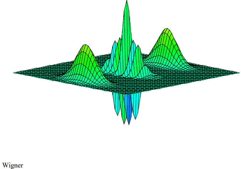
The signature of a superposition is the occurrence of interference fringes as seen in the center of the figure above.
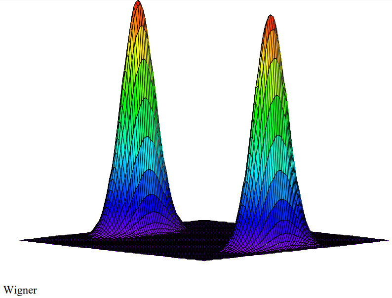
The Wigner function for a classical mixture is the sum of Wigner functions for each member of the mixture. The interference region is clearly absent in the figure shown below.
\[
\mathrm{W}(\mathrm{x}, \mathrm{p}) :=\int_{-\infty}^{\infty} \exp \left[-\left(\mathrm{x}+\frac{\mathrm{s}}{2}-5\right)^{2}\right] \cdot \exp (\mathrm{i} \cdot \mathrm{p} \cdot \mathrm{s}) \cdot \exp \left[-\left(\mathrm{x}-\frac{\mathrm{s}}{2}-5\right)^{2}\right] \mathrm{ds}+\int_{-\infty}^{\infty} \exp \left[-\left(x+\frac{s}{2}+5\right)^{2}\right] \cdot \exp (i \cdot p \cdot s) \cdot \exp \left[-\left(x-\frac{s}{2}+5\right)^{2}\right] d s
\nonumber \]
Integration yields:
\[
\mathrm{W}(\mathrm{x}, \mathrm{p}) :=\exp \left(-2 \cdot \mathrm{x}^{2}+20 \cdot \mathrm{x}-50-\frac{1}{2} \cdot \mathrm{p}^{2}\right) \cdot \sqrt{2} \cdot \sqrt{\pi}+\exp \left(-2 \cdot \mathrm{x}^{2}-20 \cdot \mathrm{x}-50-\frac{1}{2} \cdot \mathrm{p}^{2}\right) \cdot \sqrt{2} \cdot \sqrt{\pi}
\nonumber \]
\[
\mathrm{N} :=100 \qquad \mathrm{i} :=0 \ldots \mathrm{N} \qquad \mathrm{x}_{\mathrm{i}} :=-7+\frac{14 \cdot \mathrm{i}}{\mathrm{N}} \\ \mathrm{j} :=0 \ldots \mathrm{N} \qquad \mathrm{p}_{\mathrm{j}} :=-6+\frac{12 \cdot \mathrm{j}}{\mathrm{N}} \qquad \text{Wigner}_{i, j} :=\mathrm{W}\left(\mathrm{x}_{i}, \mathrm{p}_{j}\right)
\nonumber \]
Reference: Decoherence and the Transition form Quantum to Classical, Wojciech Jurek, Physics Today, October 1991, pages 36-44.