
14.1: Time-Dependent Vector Potentials
- Page ID
- 60590

\( \newcommand{\vecs}[1]{\overset { \scriptstyle \rightharpoonup} {\mathbf{#1}} } \)
\( \newcommand{\vecd}[1]{\overset{-\!-\!\rightharpoonup}{\vphantom{a}\smash {#1}}} \)
\( \newcommand{\id}{\mathrm{id}}\) \( \newcommand{\Span}{\mathrm{span}}\)
( \newcommand{\kernel}{\mathrm{null}\,}\) \( \newcommand{\range}{\mathrm{range}\,}\)
\( \newcommand{\RealPart}{\mathrm{Re}}\) \( \newcommand{\ImaginaryPart}{\mathrm{Im}}\)
\( \newcommand{\Argument}{\mathrm{Arg}}\) \( \newcommand{\norm}[1]{\| #1 \|}\)
\( \newcommand{\inner}[2]{\langle #1, #2 \rangle}\)
\( \newcommand{\Span}{\mathrm{span}}\)
\( \newcommand{\id}{\mathrm{id}}\)
\( \newcommand{\Span}{\mathrm{span}}\)
\( \newcommand{\kernel}{\mathrm{null}\,}\)
\( \newcommand{\range}{\mathrm{range}\,}\)
\( \newcommand{\RealPart}{\mathrm{Re}}\)
\( \newcommand{\ImaginaryPart}{\mathrm{Im}}\)
\( \newcommand{\Argument}{\mathrm{Arg}}\)
\( \newcommand{\norm}[1]{\| #1 \|}\)
\( \newcommand{\inner}[2]{\langle #1, #2 \rangle}\)
\( \newcommand{\Span}{\mathrm{span}}\) \( \newcommand{\AA}{\unicode[.8,0]{x212B}}\)
\( \newcommand{\vectorA}[1]{\vec{#1}} % arrow\)
\( \newcommand{\vectorAt}[1]{\vec{\text{#1}}} % arrow\)
\( \newcommand{\vectorB}[1]{\overset { \scriptstyle \rightharpoonup} {\mathbf{#1}} } \)
\( \newcommand{\vectorC}[1]{\textbf{#1}} \)
\( \newcommand{\vectorD}[1]{\overrightarrow{#1}} \)
\( \newcommand{\vectorDt}[1]{\overrightarrow{\text{#1}}} \)
\( \newcommand{\vectE}[1]{\overset{-\!-\!\rightharpoonup}{\vphantom{a}\smash{\mathbf {#1}}}} \)
\( \newcommand{\vecs}[1]{\overset { \scriptstyle \rightharpoonup} {\mathbf{#1}} } \)
\( \newcommand{\vecd}[1]{\overset{-\!-\!\rightharpoonup}{\vphantom{a}\smash {#1}}} \)
\(\newcommand{\avec}{\mathbf a}\) \(\newcommand{\bvec}{\mathbf b}\) \(\newcommand{\cvec}{\mathbf c}\) \(\newcommand{\dvec}{\mathbf d}\) \(\newcommand{\dtil}{\widetilde{\mathbf d}}\) \(\newcommand{\evec}{\mathbf e}\) \(\newcommand{\fvec}{\mathbf f}\) \(\newcommand{\nvec}{\mathbf n}\) \(\newcommand{\pvec}{\mathbf p}\) \(\newcommand{\qvec}{\mathbf q}\) \(\newcommand{\svec}{\mathbf s}\) \(\newcommand{\tvec}{\mathbf t}\) \(\newcommand{\uvec}{\mathbf u}\) \(\newcommand{\vvec}{\mathbf v}\) \(\newcommand{\wvec}{\mathbf w}\) \(\newcommand{\xvec}{\mathbf x}\) \(\newcommand{\yvec}{\mathbf y}\) \(\newcommand{\zvec}{\mathbf z}\) \(\newcommand{\rvec}{\mathbf r}\) \(\newcommand{\mvec}{\mathbf m}\) \(\newcommand{\zerovec}{\mathbf 0}\) \(\newcommand{\onevec}{\mathbf 1}\) \(\newcommand{\real}{\mathbb R}\) \(\newcommand{\twovec}[2]{\left[\begin{array}{r}#1 \\ #2 \end{array}\right]}\) \(\newcommand{\ctwovec}[2]{\left[\begin{array}{c}#1 \\ #2 \end{array}\right]}\) \(\newcommand{\threevec}[3]{\left[\begin{array}{r}#1 \\ #2 \\ #3 \end{array}\right]}\) \(\newcommand{\cthreevec}[3]{\left[\begin{array}{c}#1 \\ #2 \\ #3 \end{array}\right]}\) \(\newcommand{\fourvec}[4]{\left[\begin{array}{r}#1 \\ #2 \\ #3 \\ #4 \end{array}\right]}\) \(\newcommand{\cfourvec}[4]{\left[\begin{array}{c}#1 \\ #2 \\ #3 \\ #4 \end{array}\right]}\) \(\newcommand{\fivevec}[5]{\left[\begin{array}{r}#1 \\ #2 \\ #3 \\ #4 \\ #5 \\ \end{array}\right]}\) \(\newcommand{\cfivevec}[5]{\left[\begin{array}{c}#1 \\ #2 \\ #3 \\ #4 \\ #5 \\ \end{array}\right]}\) \(\newcommand{\mattwo}[4]{\left[\begin{array}{rr}#1 \amp #2 \\ #3 \amp #4 \\ \end{array}\right]}\) \(\newcommand{\laspan}[1]{\text{Span}\{#1\}}\) \(\newcommand{\bcal}{\cal B}\) \(\newcommand{\ccal}{\cal C}\) \(\newcommand{\scal}{\cal S}\) \(\newcommand{\wcal}{\cal W}\) \(\newcommand{\ecal}{\cal E}\) \(\newcommand{\coords}[2]{\left\{#1\right\}_{#2}}\) \(\newcommand{\gray}[1]{\color{gray}{#1}}\) \(\newcommand{\lgray}[1]{\color{lightgray}{#1}}\) \(\newcommand{\rank}{\operatorname{rank}}\) \(\newcommand{\row}{\text{Row}}\) \(\newcommand{\col}{\text{Col}}\) \(\renewcommand{\row}{\text{Row}}\) \(\newcommand{\nul}{\text{Nul}}\) \(\newcommand{\var}{\text{Var}}\) \(\newcommand{\corr}{\text{corr}}\) \(\newcommand{\len}[1]{\left|#1\right|}\) \(\newcommand{\bbar}{\overline{\bvec}}\) \(\newcommand{\bhat}{\widehat{\bvec}}\) \(\newcommand{\bperp}{\bvec^\perp}\) \(\newcommand{\xhat}{\widehat{\xvec}}\) \(\newcommand{\vhat}{\widehat{\vvec}}\) \(\newcommand{\uhat}{\widehat{\uvec}}\) \(\newcommand{\what}{\widehat{\wvec}}\) \(\newcommand{\Sighat}{\widehat{\Sigma}}\) \(\newcommand{\lt}{<}\) \(\newcommand{\gt}{>}\) \(\newcommand{\amp}{&}\) \(\definecolor{fillinmathshade}{gray}{0.9}\)The full N-electron non-relativistic Hamiltonian H discussed earlier in this text involves the kinetic energies of the electrons and of the nuclei and the mutual Coulombic interactions among these particles
\[H = \sum\limits_{a=1,M} -\left(\dfrac{\hbar^2}{2m_a}\right) \nabla_a^2 + \sum\limits_j \left[ \left(-\dfrac{\hbar^2}{2m_e}\right) \nabla_j^2 - \sum\limits_a Z_a \dfrac{e^2}{r_{j,a}} \right] + \sum\limits_{j<k}\dfrac{e^2}{r_{j,k}} + \sum\limits_{a<b}Z_aZ_b \dfrac{e^2}{R_{a,b}}. \nonumber \]
When an electromagnetic field is present, this is not the correct Hamiltonian, but it can be modified straightforwardly to obtain the proper H.
The Time-Dependent Vector \(\textbf{A}(\textbf{r},t)\) Potential
The only changes required to achieve the Hamiltonian that describes the same system in the presence of an electromagnetic field are to replace the momentum operators P\(_a\) and p\(_j\) for the nuclei and electrons, respectively, by (P\(_a\) - Z\(_a\) e/c A(R\(_a\),t)) and (p\(_j\) - e/c A(rj ,t)). Here Za e is the charge on the ath nucleus, -e is the charge of the electron, and c is the speed of light.
The vector potential A depends on time t and on the spatial location r of the particle in the following manner:
\[ \textbf{A}(\textbf{r},t) = 2 \textbf{A}_0 cos(\omega t - \textbf{k}\cdot{\textbf{r}}). \nonumber \]
The circular frequency of the radiation \(\omega\) (radians per second) and the wave vector k (the magnitude of k is |k| = \(\frac{2\pi}{\lambda}\), where \(\lambda\) is the wavelength of the light) control the temporal and spatial oscillations of the photons. The vector \(\textbf{A}_o\) characterizes the strength (through the magnitude of \(\textbf{A}_o\)) of the field as well as the direction of the A potential; the direction of propagation of the photons is given by the unit vector k/|k|. The factor of 2 in the definition of A allows one to think of \(\textbf{A}_0\) as measuring the strength of both \( e^{i(\omega t - \textbf{k}\cdot{\textbf{r}})} \) and \( e^{i(\omega t - \textbf{k}\cdot{\textbf{r}})} \) components of the \( cos(\omega t - \textbf{k}\cdot{\textbf{r}}) \) function.
The Electric \(\textbf{E}(\textbf{r},t) \text{ and Magnetic } \textbf{H}(\textbf{r},t) \text{ Fields }\)
The electric \(\textbf{E}(\textbf{r},t) \text{ and magnetic } \textbf{H}(\textbf{r}\),t) fields of the photons are expressed in terms of the vector potential A as
\[ \textbf{E}(\textbf{r},t) = -\dfrac{1}{3}\dfrac{\partial \textbf{A}}{\partial t} = \dfrac{\omega}{c}\textbf{A}_0 \sin( \omega t - \textbf{k}\cdot{\textbf{r}} ) \nonumber \]
\[ \textbf{H}(\textbf{r},t) = \nabla \textbf{ x A } = \textbf{ k x A}_o 2 \sin(\omega t - \textbf{k}\cdot{\textbf{r}}). \nonumber \]
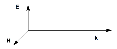
The E field lies parallel to the \(\textbf{A}_o\) vector, and the H field is perpendicular to \(\textbf{A}_o\); both are perpendicular to the direction of propagation of the light k/|k|. E and H have the same phase because they both vary with time and spatial location as \(\sin (\omega t - \textbf{k}\cdot{\textbf{r}}).\) The relative orientations of these vectors are shown below.
The Resulting Hamiltonian
Replacing the nuclear and electronic momenta by the modifications shown above in the kinetic energy terms of the full electronic and nuclear-motion hamiltonian results in the following additional factors appearing in H:
\[ H_{int} = \sum\limits_j \left[ \dfrac{ie\hbar}{m_ec}\textbf{A}(r_j,t)\cdot{\nabla_j} + \left( \dfrac{e^2}{2m_ec^2} \right)|\textbf{A}(r_j,t)|^2 \right] + \sum\limits_a \left[ \left( iZ_a\dfrac{e\hbar}{m_ac} \right)\textbf{A}(R_a,t)\cdot{\nabla_a} + \left( \dfrac{Z_a^2e^2}{2m_ac^2} \right)|\textbf{A}(R_a,t)|^2 \right]. \nonumber \]
These so-called interaction perturbations \(H_{int}\) are what induces transitions among the various electronic/vibrational/rotational states of a molecule. The one-electron additive nature of \(H_{int}\) plays an important role in determining the kind of transitions that \(H_{int}\) can induce. For example, it causes the most intense electronic transitions to involve excitation of a single electron from one orbital to another (e.g., the Slater-Condon rules).