4.5: Group Theory Considerations

Group theory provides a powerful set of tools for predicting and interpreting vibrational spectra. In this section, we will consider how Group Theory helps us to understand these important phenomena.

Transformation of Axes and Rotations

It is possible to determine the symmetry species or irreducible representation by which each of the three Cartesian coordinate axes transform. This is useful, particularly in determining selection rules in spectroscopy, as the components of a molecule’s dipole moment will transform as these axes. The rotations are also useful in understanding the rotational selection rules.

Recall the character table for the \(C_{2v}\) point group.

\(C_{2v}\)	E	\(C_{2}\)	\(\sigma_{v}\)	\(\sigma_ {v}\) ’
\(A_ {1}\)	1	1	1	1
\(A_ {2}\)	1	1	-1	-1
\(B_ {1}\)	1	-1	1	-1
\(B_ {2}\)	1	-1	-1	1

It is useful to determine how each axis (x, y and z) is transformed under each symmetry operation. Once this is done, it will be easy to determine the representation that transforms the axis in this way. A table might be useful. Recalling our designation of the \(\sigma_ {v}\) operation as reflection through the xz plane, it can be shown easily that the axes transform as follows:

\(C_ {2v}\)	E	\(C_ {2}\)	\(\sigma_ {v}\)	\(\sigma_ {v}\) ’
x	x	-x	x	-x
y	y	-y	-y	y
z	z	z	z	z

The z-axis is unchanged by any of the symmetry operations. Another way of saying this is that the z-axis is symmetric with respect to all of the operations. (In this point group, all of the symmetry elements happen to intersect on the z-axis, which is why it is unchanged by any of the symmetry operations.) The conclusion is that the z-axis transforms with the \(A_ {1}\) representation.

The other axes can be described the same way. Note that the x-axis is symmetric with respect to the \(\sigma_ {v}\) operation and the E operation. (Everything is symmetric with respect to the E operation, oddly enough.) The x-axis is antisymmetric, however, with respect to the \(\sigma_ {v}\) ’ and \(C_ {2}\) operations. The results for all axes can be summarized in the character table.

\(C_ {2v}\)	E	\(C_ {2}\)	\(\sigma_ {v}\)	\(\sigma_ {v}\) ’
\(A_ {1}\)	1	1	1	1	z
\(A_ {2}\)	1	1	-1	-1
\(B_ {1}\)	1	-1	1	-1	x
\(B_ {2}\)	1	-1	-1	1	y

Rotations about the x, y and z axes can be characterized in a similar fashion. Consider the angular momentum vector for each rotation and how it transforms. Such a vector can be constructed using he right-hand rule. If the fingers on your right hand point in the direction of the rotation, your thumb points in the direction of the angular momentum vector.

Rotation about the z-axis (\(R_ {z}\) ) is symmetric with respect to the operations E and \(C_ {2}\), but antisymmetric with respect to operations \(\sigma_ {v}\) and \(\sigma_ {v}\) ’. Rotation about the x-axis is symmetric with respect to E and \(C_ {2}\). Clearly, this operation transforms as the irreducible representation \(A_ {2}\). Rotation about the x-axis and y-axis can also be characterized as following the properties of the \(B_ {2}\) and \(B_ {1}\) representations respectively. As such, the character table for \(C_ {2v}\) can be augmented to include this information.

\(C_ {2v}\)	E	\(C_ {2}\)	\(\sigma_ {v}\)	\(\sigma_ {v}\) ’
\(A_ {1}\)	1	1	1	1	z
\(A_ {2}\)	1	1	-1	-1		\(R_ {z}\)
\(B_ {1}\)	1	-1	1	-1	x	\(R_ {y}\)
\(B_ {2}\)	1	-1	-1	1	y	\(R_ {x}\)

Another interpretation of the transformation of the x, y and z-axes is that the representations that indicate the symmetries of these axes in the point group also indicate how the \(p_ {x}\), \(p_ {y}\) and \(p_ {z}\) orbitals transform. The set of d orbital wavefunctions can also be used. These transformations are generally given in another column in the character table. (This information is also useful for calculating polarizabilities, and hence selection rules for Raman transitions!)

\(C_ {2v}\)	E	\(C_ {2}\)	\(\sigma_ {v}\)	\(\sigma_ {v}\) ’
\(A_ {1}\)	1	1	1	1	z		\(x ^{2}\) -\(y ^{2}\), \(z ^{2}\)
\(A_ {2}\)	1	1	-1	-1		\(R_ {z}\)	xy
\(B_ {1}\)	1	-1	1	-1	x	\(R_ {y}\)	xz
\(B_ {2}\)	1	-1	-1	1	y	\(R_ {x}\)	yz

Characterizing Vibrational Modes

Vibrational wave functions describing the normal modes of vibrations will be eigenfunctions of the symmetry properties of the group. As such, group theory can be quite useful in determining the vibrational selection rules needed to predict infrared spectra.

The number of vibrational degrees of freedom for a molecule is given by (\(3N-6\)) if the molecule is non-linear and (\(3N-5\)) if it is linear. In these expressions, N is the number of atoms in the molecule. One way to think of these numbers is that it takes 3N Cartesian coordinates (an x, y and z variable) for each atom in the molecule to fully specify the structure of a molecule. As such, 3N is the total number of degrees of freedom.

Since the molecule can translate through space in the x, y or z directions, three (3) degrees of freedom belong to translation. One can also think of these three degrees of freedom being the three Cartesian coordinates needed to specify the location of the center of mass of the molecule – or for the translation of the center of mass of the molecule.

For non-linear molecules, rotation can occur about each of the three Cartesian axes as well. So three (3) degrees of freedom belong to rotation for non-linear molecules. Linear molecules only have rotational degrees of freedom about the two axes that are perpendicular to the molecular axis (which remember is the C axis – and thus the z-axis.) So linear molecules only have two (2) rotational degrees of freedom.

The sum of the irreducible representations by which the vibrational modes transform can be found fairly easily using group theory. The first step is to determine how the three Cartesian axes transform under the symmetry operations of the point group. As an example, let’s use water (\(H_ {2} O\)), which belongs to the \(C_ {2v}\) point group since it is familiar. Later, we will work though a more complex example.

Consider the character table for the \(C_ {2v}\) point group.

\(C_ {2v}\)	E	\(C_ {2}\)	\(\sigma_ {v}\)	\(\sigma_ {v}'\)
\(A_ {1}\)	1	1	1	1	z		\(x ^{2} -y ^{2}\), \(z ^{2}\)
\(A_ {2}\)	1	1	-1	-1		\(R_ {z}\)	xy
\(B_ {1}\)	1	-1	1	-1	x	\(R_ {y}\)	xz
\(B_ {2}\)	1	-1	-1	1	y	\(R_ {x}\)	yz

The sum of the representations by which the axes transform will be given by \(B_ {1} + B_ {2} + A_ {1}\).

\(C_ {2v}\)		E	\(C_ {2}\)	\(\sigma_ {v}\)	\(\sigma_ {v}\) ’
\(\Gamma_ {1}\)	\(A_ {1}\)	1	1	1	1	z
\(\Gamma_ {2}\)	\(B_ {1}\)	1	-1	1	-1	x
\(\Gamma_ {3}\)	\(B_ {2}\)	1	-1	-1	1	y
\(\Gamma_ {xyz}\)	\(A_1 + B_1 + B_2\)	3	-1	1	1

The reducible representation (\(\Gamma_ {xyz}\) ) is then multiplied by the representation generated by counting the number of atoms in the molecule that remain unmoved by each symmetry element. This representation for water is generated as follows:

\(C_ {2v}\)	E	\(C_ {2}\)	\(\sigma_ {v}\)	\(\sigma_ {v}\) ’
\(O\)	\(\checkmark\)	\(\checkmark\)	\(\checkmark\)	\(\checkmark\)
\(H_ {1}\)	\(\checkmark\)	-	-	\(\checkmark\)
\(H_ {2}\)	\(\checkmark\)	-	-	\(\checkmark\)
\(\Gamma_ {unmoved}\)	3	1	1	3

Figure \(\PageIndex{1}\)

The reducible representation that describes the transformation of the Cartesian coordinates of each of the atoms in the molecule are given by the product of \(\Gamma_ {xyz} \cdot\Gamma_ {unmoved}\) as shown in the following table.

\(C_ {2v}\)	E	\(C_ {2}\)	\(\sigma_ {v}\)	\(\sigma_ {v}\) ’
\(\Gamma_ {xyz}\)	3	-1	1	1
\(\Gamma_ {unmoved}\)	3	1	1	3
\(\Gamma_ {total} = \Gamma_ {xyz} \cdot\Gamma_ {unmoved}\)	9	-1	1	3

Note that the order of \(\Gamma_ {total}\) is given by \(3N\). This is the sum of representations needed to describe the transformation of each of the Cartesian coordinates for each atom. f the representation for the Cartesian coordinates (\(\Gamma_ {xyz}\) ) is subtracted from \(\Gamma_ {total}\), the remainder describes the sum of representations by which the rotations and vibrations transform, and this result should be of order (\(3N-3\)). Let’s see . . .

\(C_ {2v}\)	E	\(C_ {2}\)	\(\sigma_ {v}\)	\(\sigma_ {v}\) ’
\(\Gamma_ {total}\)	9	-1	1	3
\(\Gamma_ {xyz}\)	3	-1	1	1
\(\Gamma_ {vib+rot}\)	6	0	0	2

So far, so good. Now let’s subtract the sum of the representations by which the rotations transform. The remainder of this operation should be of order (\(3N-6\)) and give the sum of irreducible representations by which the vibrations transform.

\(C_{2v}\)	E	\(C_ {2}\)	\(\sigma_ {v}\)	\(\sigma_ {v}\) ’
\(\Gamma_{vib+rot}\)	6	0	0	2
\(\Gamma_{rot}\)	3	-1	-1	-1
\(\Gamma_{vib}\)	3	1	1	3

\(C_ {2v}\)	E	\(C_ {2}\)	\(\sigma_ {v}\)	\(\sigma_ {v}\) ’
\(A_ {1}\)	1	1	1	1
\(A_ {1}\)	1	1	1	1
\(B_ {2}\)	1	-1	-1	1
\(\Gamma_ {vib}\)	3	1	1	3

A quick calculation shows that this result is generated by the sum of \(A_ {1}\) + \(A_ {1}\) + \(B_ {2}\). To see this, we can use the Great Orthogonality Theorem. (I told you it was great!) In this case, the number of vibrational modes that transform as the \(i^{th}\) irreducible representation is given by the relationship \[N_{i} =\dfrac{1}{h} \sum _{R}\chi _{i} (R)\chi _{vib} (R)\nonumber\]

For the \(A_ {1}\) representation, this sum looks as follows.

\[\begin{array}{rcl} {N{}_{A_{1} } } & {=} & {\dfrac{1}{h} \left(\chi _{A_{1} } (E)\cdot \chi _{vib} (E)+\chi _{A_{1} } (C_{2} )\cdot \chi _{vib} (C_{2} )+\chi _{A_{1} } (\sigma _{v} )\cdot \chi _{vib} (\sigma _{v} )+\chi _{A_{1} } (\sigma _{v}^{'} )\cdot \chi _{vib} (\sigma _{v}^{'} )\right)} \\ {} & {=} & {\dfrac{1}{4} \left((1)\cdot (3)+(1)\cdot (1)+(1)\cdot (1)+(1)\cdot (3)\right)} \\ {} & {=} & {\dfrac{1}{4} \left(8\right)} \\ {} & {=} & {2} \end{array}\nonumber\]

The result for the \(A_ {2}\) representation should come to zero since no vibrational modes transform as \(A_ {2}\). For the \(A_ {2}\) representation, this sum looks as follows.

\[\begin{array}{rcl} {N_{A_{2} } } & {=} & {\dfrac{1}{4} \left((1)\cdot (3)+(1)\cdot (1)+(-1)\cdot (1)+(-1)\cdot (3)\right)} \\ {} & {=} & {\dfrac{1}{4} \left(0\right)=0} \end{array}\nonumber\]

For \(B_ {1}\) and \(B_ {2}\) the sum looks as follows:

\[\begin{array}{rcl} {N_{B_{1} } } & {=} & {\dfrac{1}{4} \left((1)\cdot (3)+(-1)\cdot (1)+(1)\cdot (1)+(-1)\cdot (3)\right)} \\ {} & {=} & {\dfrac{1}{4} \left(0\right)=0} \end{array}\nonumber\]

\[\begin{array}{rcl} {N_{B_{2} } } & {=} & {\dfrac{1}{4} \left((1)\cdot (3)+(-1)\cdot (1)+(-1)\cdot (1)+(1)\cdot (3)\right)} \\ {} & {=} & {\dfrac{1}{4} \left(4\right)=1} \end{array}\nonumber\]

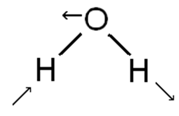
Let’s see if that makes sense! Consider the three normal-mode vibrations in water. These (the symmetric stretch, the bend and the antisymmetric stretch) can be depicted as follows:

It is fairly simple to show that the symmetric stretch and the bending mode both transform as the \(A_ {1}\) representation. Similarly, the antisymmetric stretching mode transforms as the \(B_ {2}\) representation. (Note that we have chosen the xz plane (or the \(\sigma_ {v}\) plane) to lie perpendicular to the molecule!)

Figure \(\PageIndex{2}\)

Example \(\PageIndex{1}\)

Find the symmetries of the normal vibrational modes of ammonia.

Solution

Recall the character table for the \(C_ {3v}\) point group:

\(C_{3v}\)	E	2 \(C_{3}\)	3 \sigma
\(A_1\)	1	1	1	z
\(A_2\)	1	1	-1		\(R_z\)
E	2	-1	0	\(x\), \(y\)	\(R_x\), \(R_y\)

The representation for \(\Gamma_ {total}\) can be found in the same way as before. Once we have \(\Gamma_ {total}\), \(\Gamma_ {vib}\) is determined as before.

\(C_{3v}\)	E	2 \(C_{3}\)	3\(\sigma_{v}\)
\(\Gamma_{xyz}\)	3	1	1
\(\Gamma_{unmoved}\)	4	1	2
\(\Gamma_{total}\)	12	1	2

\(C_{3v}\)	E	2 \(C_{3}\)	3\(\sigma_{v}\)
\(\Gamma_{total}\)	12	1	2
\(\Gamma_{xyz}\)	3	1	1
\(\Gamma_{rot}\)	3	0	-1
\(\Gamma_{vib}\)	6	0	2

The GOT can be used to find how many modes of each symmetry are present.

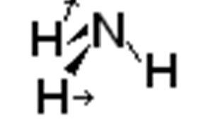
Mode		Freq. (cm^-1)	Sym.
Umbrella		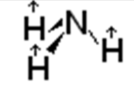1139	\(A_1\)
Bend		1765	E
Antisym. Str.		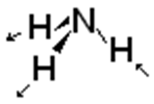3464	E
Sym. Str.		3534	\(A_1\)

\[\begin{aligned}
N_{A_1} & =\dfrac{1}{6}[(1) \cdot(6)+2(1) \cdot(0)+3(1) \cdot(2)] \\
& =\dfrac{1}{6}(12)=2
\end{aligned}\nonumber\]

\[\begin{aligned}
N_{A_2} & =\dfrac{1}{6}[(1) \cdot(6)+2(1) \cdot(0)+3(-1) \cdot(2)] \\
& =\dfrac{1}{6}(0)=0
\end{aligned}\nonumber\]

\[\begin{aligned}
N_E & =\dfrac{1}{6}[(2) \cdot(6)+2(-1) \cdot(0)+3(0) \cdot(2)] \\
& =\dfrac{1}{6}(12)=2
\end{aligned}\nonumber\]

So there are two (2) \(A_ {1}\) modes and two (2) doubly degenerate E modes of vibration. These can be summarized in the table to the right.

Example \(\PageIndex{2}\): The vibrational modes of \(SF_4\)

Figure \(\PageIndex{3}\)

Solution

\(SF _{4}\) is an example of a molecule with a “see saw” geometry. It belongs to the point group \(C_ {2v}\) like water. Let’s find the symmetries of the normal modes of vibration using group theory. First, we must generate \(\Gamma_ {total}\).

\(C_{2v}\)	E	\(C_{2}\)	\(\sigma_{v}\)	\(\sigma_{v}\)’
\(\Gamma_{xyz}\)	3	-1	1	1
\(\Gamma_{unmoved}\)	5	1	3	3
\(\Gamma_{total}\)	15	-1	3	3

\(C_{2v}\)	E	\(C_{2}\)	\(\sigma_{v}\)	\(\sigma_{v}\)’
\(\Gamma_{total}\)	15	-1	3	3
\(\Gamma_{xyz}\)	3	-1	1	1
\(\Gamma_{rot}\)	3	-1	-1	-1
\(\Gamma_{vib}\)	9	1	3	3

Now, subtract \(\Gamma_ {xyz}\) and \(\Gamma_ {rot}\) to generate \(\Gamma_ {vib}\) as shown above.

So this implies that there are nine degrees of freedom due to vibration. This is the result we expect since for the 5-atom non-linear molecule, (3N-6) = 9. To generate the number of vibrational modes that transform as the \(A_ {1}\) irreducible representation, the follow expression must be evaluated.

\[\begin{aligned}
N_{A_1} & =\dfrac{1}{h}\left(\chi_{A_1}(E) \cdot \chi_{v i b}(E)+\chi_{A_1}\left(C_2\right) \cdot \chi_{v i b}\left(C_2\right)+\chi_{A_1}\left(\sigma_v\right) \cdot \chi_{v i b}\left(\sigma_v\right)+\chi_{A_1}\left(\sigma_v^{\prime}\right) \cdot \chi_{v i b}\left(\sigma_v^{\prime}\right)\right) \\
& =\dfrac{1}{4}((1) \cdot(9)+(1) \cdot(1)+(1) \cdot(3)+(1) \cdot(3)) \\
& =\dfrac{1}{4}(16) \\
& =4
\end{aligned}\nonumber\]

Similarly,

\[\begin{aligned}
N_{A_2} & =\dfrac{1}{4}((1) \cdot(9)+(1) \cdot(1)+(-1) \cdot(3)+(-1) \cdot(3)) \\
& =\dfrac{1}{4}(4)=1
\end{aligned}\nonumber\]

\[\begin{aligned}
N_{B_1} & =\dfrac{1}{4}((1) \cdot(9)+(-1) \cdot(1)+(1) \cdot(3)+(-1) \cdot(3)) \\
& =\dfrac{1}{4}(8)=2
\end{aligned}\nonumber\]

\[\begin{aligned}
N_{B_2} & =\dfrac{1}{4}((1) \cdot(9)+(-1) \cdot(1)+(-1) \cdot(3)+(1) \cdot(3)) \\
& =\dfrac{1}{4}(8)=2
\end{aligned}\nonumber\]

So there should be 4 vibrational modes of \(A_ {1}\) symmetry, 1 of \(A_ {2}\) symmetry and two each of \(B_ {1}\) and \(B_ {2}\) symmetry. A calculation of the structure and vibrational frequencies in \(SF _{4}\) at the B3LYP/6-31G(d) level of theory¹ yields the following.

Mode	Freq. (cm^-1)	Symmetry	Mode	Freq. (cm^-1)	Symmetry
1	189	\(A_1\)	6	584	\(A_1\)
2	330	\(B_1\)	7	807	\(B_2\)
3	436	\(A_2\)	8	852	\(B_1\)
4	487	\(A_1\)	9	867	\(A_1\)
5	496	\(B_2\)

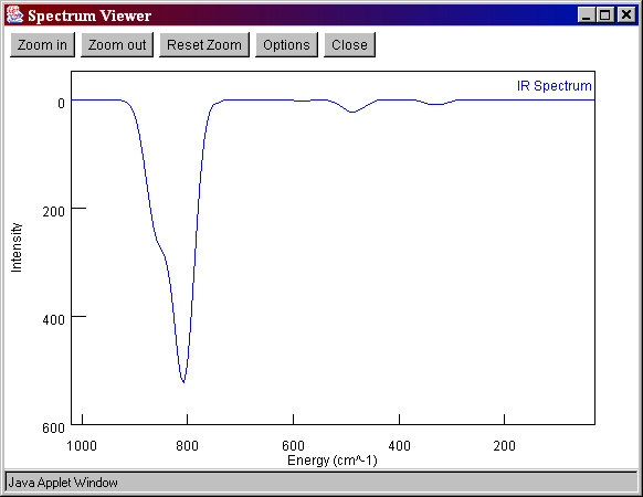
The calculation also allows for the simulation of the infrared spectrum of \(SF _{4}\).

Figure \(\PageIndex{4}\)

What would be exceptionally useful is if group theory could help to identify which vibrational modes are active – or if any are inactive. Fortunately, it can! (And now how much would you pay?) The tools for determining selection rules depend on direct products.

Intensity

Group theory provides tools to calculate when a spectral transition will have zero intensity, and this will not be seen. In this section, we will se how group theory can help to determine the selection rules that govern which transitions can and cannot be see.

\(\text{Intensity} \propto \left|\int \left(\psi '\right)^{*} \vec{\mu }\left(\psi "\right) d\tau \right|^{2}\)

The intensity of a transition in the spectrum of a molecule is proportional to the magnitude squared of the transition moment matrix element.

By knowing the symmetry of each part of the integrand, the symmetry of the product can be determined as the direct product of the symmetries of each part (\psi’) \({}^{*}\), (\psi”) and \mu. This is helpful, since the integrand must not be antisymmetric with respect to any symmetry elements or the integral will vanish by symmetry. Before exploring that concept, lets look at the concept of direct products.

This is a concept many people have seen, in that the integral of an odd function over a symmetric interval, is zero. Recall what it means to be an “odd function” or an “even function.

Symmetry	definition	Intensity
Even	\(f(-x) = f(x)\)	\(\int _{-a}^{a}f(x)dx=2\int _{0}^{a}f(x)dx\)
Odd	\(f(-x) = -f(x)\)	\(\int _{-a}^{a}f(x)dx=0\)

Consider the function \(f(x)=\left(x^{3} -3x\right)e^{-x^{2} }\). A graph of this function looks as follows:

One notes that the area under the curve on the side of the function for which x \(\mathrm{>}\) 0 has exactly the same magnitude but opposite sign of the area under the other side of the graph. Mathematically,

\[\begin{array}{rcl} {\int _{-a}^{a}f(x)dx } & {=} & {\int _{-a}^{0}f(x)dx +\int _{0}^{a}f(x)dx } \\ {} & {} & {=-\int _{0}^{a}f(x)dx +\int _{0}^{a}f(x)dx =0} \end{array}\nonumber\]

It is also interesting to note that the function f(x) can be expressed as the product of two functions, one of which is an odd function ( \(x^{3} -3x\) ) and the other which is an even function ( \(e^{-x^{2} }\) ). The result is an odd function. By determining the symmetry of the function as a product of the eigenvalues of the functions with respect to the inversion operator, as discussed below, one can derive a similar result.

The even/odd symmetry is an example of inversion symmetry. Recall that the inversion operator (in one dimension) affects a change of sign on x.

\[\hat{i}f(x)=f(-x)\nonumber\]

“Even” and “odd” functions are eigenfunctions of this operator, and have eigenvalues of either +1 or –1. For the function used in the previous example,

\[f(x)=g(x)h(x)\nonumber\]

where

\(g(x)=x^{3} -3x\) and \(h(x)=e^{-x^{2} }\)

Here, \(g(x)\) is an odd function and \(h(x)\) is an even function. The product is an odd function. This property is summarized for any \(f(x)=g(x)h(x)\), in the following table.

g(x)	h(x)	f(x)	ig(x)=__g(x)	ih(x)=__h(x)	if(x)=__f(x)
even	even	even	1	1	1
even	odd	odd	1	-1	-1
odd	odd	even	-1	-1	1

Note that the eigenvalue (+1 or –1) is simply the character of the inversion operation for the irreducible representation by which the function transforms! In a similar manner, any function that can be expressed as a product of functions (like the integrand in the transition moment matrix element) can be determined as the direct product of the irreducible representations by which each part of the product transforms.

Consider the point group \(C_ {2v}\) as an example. Recall the character table for this point group.

\(C_ {2v}\)	E	\(C_ {2}\)	\(\sigma_ {v}\)	\(\sigma_ {v}\) ’
\(A_ {1}\)	1	1	1	1	z		\(x ^{2}\) -\(y ^{2}\), \(z ^{2}\)
\(A_ {2}\)	1	1	-1	-1		\(R_ {z}\)	xy
\(B_ {1}\)	1	-1	1	-1	x	\(R_ {y}\)	xz
\(B_ {2}\)	1	-1	-1	1	y	\(R_ {x}\)	yz

The direct product of irreducible representations can by the definition

\[\chi _{prod} (R)=\chi _{i} (R)\cdot \chi _{j} (R)\nonumber\]

So for the direct product of \(B_ {1}\) and \(B_ {2}\), the following table can be used.

\(C_ {2v}\)	E	\(C_ {2}\)	\(\sigma_ {v}\)	\(\sigma_ {v}\) ’
\(B_ {1}\)	1	-1	1	-1
\(B_ {2}\)	1	-1	-1	1
\(B_ {1}\) \(\otimes\) \(B_ {2}\)	1	1	-1	-1

The product is actually the irreducible representation given by \(A_ {2}\) ! As it turns out, the direct product will always yield a set of characters that is either an irreducible representation of the group, or can be expressed as a sum of irreducible representations. This suggests that a multiplication table can be constructed. An example (for the \(C_ {2v}\) point group) is given below.

\(C_ {2v}\)	\(A_ {1}\)	\(A_ {2}\)	\(B_ {1}\)	\(B_ {2}\)
\(A_ {1}\)	\(A_ {1}\)	\(A_ {2}\)	\(B_ {1}\)	\(B_ {2}\)
\(A_ {2}\)	\(A_ {2}\)	\(A_ {1}\)	\(B_ {2}\)	\(B_ {1}\)
\(B_ {1}\)	\(B_ {1}\)	\(B_ {2}\)	\(A_ {1}\)	\(A_ {2}\)
\(B_ {2}\)	\(B_ {2}\)	\(B_ {1}\)	\(A_ {2}\)	\(A_ {1}\)

Studying this table reveals some useful generalizations. Two things in particular jump from the page. These are summarized in the following tables.

	A	B					1	2
A	A	B				1	1	2
B	B	A				2	2	1

This pattern might seem obvious to some. It stems from the idea that

symmetric*symmetric = symmetric

symmetric*antisymmetric = antisymmetric

antisymmetric*antisymmetric = symmetric

Noting that A indicates an irreducible representation is symmetric with respect to the \(C_ {2}\) operation and B indicates that the irreducible representation is antisymmetric . . and that the subscript 1 indicates that an irreducible representation is symmetric with respect to the \(\sigma_ {v}\) operation, and that a subscript 2 indicates that the irreducible representation is antisymmetric . . the rest seems to follow! Some point groups have irreducible representations use subscripts g/u or primes and double primes. The g/u subscript indicates symmetry with respect to the inversion (i) operator, and the prime/double prime indicates symmetry with respect to a \(\sigma\) plane (generally the plane of the molecule for planar molecules).

This method works well for singly degenerate representations. But what does one do for products involving doubly degenerate representations? As an example, consider the \(C_ {3v}\) point group.

\(C_ {3v}\)	E	2 \(C_ {3}\)	3\(\sigma_ {v}\)
\(A_ {1}\)	1	1	1	z
\(A_ {2}\)	1	1	-1		\(R_ {z}\)
E	2	-1	0	(x, y)	(\(R_ {x}\), \(R_ {y}\) )
\(C_ {3v}\)	E	2 \(C_ {3}\)	3\(\sigma_ {v}\)
\(A_ {2}\)	1	1	-1
E	2	-1	0
\(A_ {2}\) \(\otimes\) E	2	-1	0

Consider the direct product of \(A_ {2}\) and E.

This product is clearly just the E representation. Now one other example – Consider the product \(E \otimes E\).

\(C_ {3v}\)	E	2 \(C_ {3}\)	3\(\sigma_ {v}\)
E	2	-1	0
E	2	-1	0
\(E \otimes E\)	4	1	0

To find the irreducible representations that comprise this reducible representation, we proceed in the same manner as determining the number of vibrational modes belonging to each symmetry.

\[\begin{array}{rcl} {N_{A_{1} } } & {=} & {\dfrac{1}{6} \left[(1)(4)+2(1)(1)+3(1)(0)\right]=1} \\ {N_{A_{2} } } & {=} & {\dfrac{1}{6} \left[(1)(4)+2(1)(1)+3(-1)(0)\right]=1} \\ {N_{E} } & {=} & {\dfrac{1}{6} \left[(2)(4)+2(-1)(1)+3(0)(0)\right]=1} \end{array}\nonumber\]

This allows us to build a table of direct products. Notice that the direct product always has the total dimensionality that is given by the product of the dimensions.

\(C_ {3v}\)	\(A_ {1}\)	\(A_ {2}\)	E
\(A_ {1}\)	\(A_ {1}\)	\(A_ {2}\)	E
\(A_ {2}\)	\(A_ {2}\)	\(A_ {1}\)	E
E	E	E	\(A_ {1} + A_ {2} +E\)

Now that we have a handle on direct products, we can move on to selection rules.

Selection Rules

According to quantum mechanics, transitions will only be allowed (have non-zero intensity) if the squared magnitude of the transition moment ( \(\left|\int \psi '* \vec{\mu }\psi "d\tau \right|^{2}\) ) is not zero. If the integral vanishes by symmetry, obviously the transition moment will have zero magnitude and the transition is forbidden and will not be seen. In order to determine if the integral vanishes by symmetry, it is necessary to determine the symmetry by which the dipole moment operator transforms.

This ( \(\vec{\mu }\) ) is a vector operator and can be decomposed into \(x\), \(y\) and \(z\) components. As such, the transition moment is also a vector property that can have x-, y- and/or z-axis components. Clearly, it will be important to determine how the three axes transform. Fortunately, this information is contained in character tables! Consider the following two point groups, \(C_ {3v}\) and \(C_ {2v}\).

\(C_ {3v}\)	E	2 \(C_ {3}\)	3\(\sigma_ {v}\)
\(A_ {1}\)	1	1	1	\(z\)
\(A_ {2}\)	1	1	-1		\(R_z\)
E	2	-1	0	\((x,y)\)	\((R_x, R_y)\)

\(C_ {2v}\)	E	\(C_ {2}\)	\(\sigma_ {v}\)	\(\sigma_ {v}\) ’
\(A_ {1}\)	1	1	1	1	z
\(A_ {2}\)	1	1	-1	-1		\(R_ {z}\)
\(B_ {1}\)	1	-1	1	-1	x	\(R_ {y}\)
\(B_ {2}\)	1	-1	-1	1	Y	\(R_ {x}\)

In the case of \(C_ {2v}\), it is clear that the x-, y- and z-axes transform as the \(B_ {1}\), \(B_ {2}\) and \(A_ {1}\) irreducible representations respectively. In the case of \(C_ {3v}\), the z-axis transforms as \(A_ {1}\), but the x- and y-axes come as a pair and transform as the E irreducible representation. It will always require two axes to complete the basis for a doubly degenerate representation.

Under the \(C_ {2v}\) point group, any vector quantity will transform as the sum of \(A_ {1}\) +\(B_ {1}\) +\(B_ {2}\) as we saw for \(\Gamma_ {xyz}\) before. Further, one can say that the x-axis component transforms as \(B_ {1}\), the y-axis component as \(B_ {2}\) and the z-axis component as \(A_ {1}\). By a similar token, under the \(C_ {3v}\) point group, a vector quantity transforms as the sum of \(A_ {1} +E\). The z-axis component transforms as \(A_ {1}\) and the x- and y-axis components come as a pair that transform by the E representation. All that is needed to complete the picture is to determine the symmetries of the upper and lower state wave functions.

Infrared Active Transitions

In order for a spectral transition to be allowed by electric dipole selection rules, the transition moment integral must not vanish.

\[\int \psi '^{*} \vec{\mu }\psi " d\tau\nonumber\]

This can be determined by using the irreducible representations by which the two wavefunctions transform and the three components of the transition moment operator, which will be \(x\), \(y\) and \(z\).

\[\int \Gamma _{\psi '} \Gamma _{\vec{\mu }} \Gamma _{\psi "} d\tau\nonumber\]

If the direct product of the integrand does not contain at least a component of the totally symmetric irreducible representation, the integral will vanish by symmetry.

Example \(\PageIndex{3}\)

The three vibrational modes of \(H_ {2}\) O transform by \(A_ {1}\) (symmetric stretch), \(A_ {1}\) (bend) and \(B_ {2}\) (antisymmetric stretch.) Will the symmetric stretch mode be infrared active?

Solution

For the symmetric stretch, which transforms as \(A_ {1}\), the transition moment integrand will be have symmetry properties determined by the product

\(\psi '\left(\begin{array}{c} {x} \\ {y} \\ {z} \end{array}\right)\psi " \qquad A_{1} \left(\begin{array}{c} {B_{1} } \\ {B_{2} } \\ {A_{1} } \end{array}\right) A_{1}\)

where one of the irreducible representations from the set in the middle of the product may be used. (They are the irreducible representations by which the \(x\), \(y\) and \(z\) axes transform.) In this case, the z-axis must be used.

\(A_ {1} \cdot A_ {1} \mathrm{\cdot} A_ {1} = A_ {1}\)

This is the only component that will not vanish.When the z-axis component must be used to make the transition moment operator not vanish, the transition is said to be a parallel transition. Transition moments that lie along axis perpendicular to the z-axis are said to be perpendicular transitions. Parallel and Perpendicular Transitions often have very different selection rules and thus very different band contours.

Another Method

Another method that can be used to see if a mode is infrared active is to take the direct product of the irreducible representations of the wavefunction, and use \(\Gamma_ {xyz}\) for the transition moment. If the resulting product has a component that is totally symmetric, the mode will be infrared active.

Example \(\PageIndex{4}\)

Is the antisymmetric stretch mode of water predicted to be infrared active?

Solution

This mode transforms as the \(B_ {2}\) irreducible representation. \(\Gamma_ {xyz}\) is given by

\(\Gamma_ {xyz} = B_ {1} + B_ {2} + A_ {1}\)

So:

\(C_{2v}\)	E	\(C_{2}\)	\(\sigma_{xz}\)	\(\sigma_{yz}\)
\(B_2\)	1	-1	-1	1
\(\Gamma_{xyz}\)	3	-1	1	1
\(\Gamma_{prod}\)	3	1	-1	1

The resulting reducible representation will have a component of the totally symmetric irreducible representation.

\(A_ {1} \cdot \Gamma_ {prod} = (1)(3) + (1)(1) + (1)(-1) + (1)(1) = 4\)

So the \(A_ {1}\) irreducible representation appears once in the product reducible representation. In fact, the component that does not vanish is due to the presence of \(B_ {2}\) in \(\Gamma_ {xyz}\). Hence, the transition is predicted to be a perpendicular \(\bot\) transition, since the transition moment lies along the y-axis.

Example \(\PageIndex{5}\)

Will the E modes in \(NH_ {3}\) be infrared active?

Solution

In the \(C_ {3v}\) point group, \(\Gamma_ {xyz}\) is given by \(A_ {1} + E\)

\(C_{3v}\)	E	2 \(C_{3}\)	3 \(\sigma_{v}\)
E	2	-1	0
\(\Gamma_{xyz}\)	3	0	1
\(\Gamma_{prod}\)	6	0	0

\(\Gamma_ {prod}\) clearly has the totally symmetric irreducible representation as a component.

\(A_1 \cdot \Gamma_{prod} = (1)(6) + 2(1)(0) + 3(1)(0) = 6\)

In fact, it is the E component of \(\Gamma_ {xyz}\) that makes this transition allowed (and so it is a perpendicular ( \(\bot\) ) transition.

\(C_{3v}\)	E	2 \(C_{3}\)	3 \(\sigma_{v}\)
E	2	-1	0
E	2	-1	0
\(\Gamma_{prod}\)	4	1	0

\(A_1 \cdot \Gamma_{prod} =(1)(4) + 2(1)(1) + 3(1)(0) = 6\)

Vibrational Raman Spectra

Vibrational Raman spectroscopy is often used as a complementa\(R_y\) method to infrared spectroscopy. The selection rules for Raman spectroscopy can be determined in much the same way, except that a polarizability integral must be used. The polarizability operator can be expressed as a 3x3 tensor of the form

\[\alpha =\left(\begin{array}{ccc} {\alpha _{xx} } & {\alpha _{xy} } & {\alpha _{xz} } \\ {\alpha _{yx} } & {\alpha _{yy} } & {\alpha _{yz} } \\ {\alpha _{zx} } & {\alpha _{zy} } & {\alpha _{zz} } \end{array}\right)\nonumber\]

This tensor is symmetric along the diagonal, and the elements transform in the same ways as the functions \(x ^{2}\), \(y ^{2}\), \(z ^{2}\), \(xy\), \(xz\) and \(yz\).

Example \(\PageIndex{6}\)

What are the vibrational mode symmetries for the molecule \(H_ {2} CCH_ {2}\) which transforms as the D \({}_{2h}\) point group? Which modes will be infrared active? Which will be Raman active?

Solution

Set up the vibrational analysis table in the usual manner.

\(D_{2h}\)	E	\(C_{2}\)(z)	\(C_{2}\)(y)	\(C_{2}\)(x)	i	\(\sigma_{xy}\)	\(\sigma_{xz}\)	\(\sigma_{yz}\)
\(A_{g}\)	1	1	1	1	1	1	1	1		\(x^2,\; y^2, \;z^2\)
\(B_{1g}\)	1	1	-1	-1	1	1	-1	-1	\(R_z\)	\(xy\)
\(B_{2g}\)	1	-1	1	-1	1	-1	1	-1	\(R_y\)	\(xz\)
\(B_{3g}\)	1	-1	-1	1	1	-1	-1	1	\(R_x\)	\(yz\)
\(A_{u}\)	1	1	1	1	-1	-1	-1	-1
\(B_{1u}\)	1	1	-1	-1	-1	-1	1	1	\(z\)
\(B_{2u}\)	1	-1	1	-1	-1	1	-1	1	\(y\)
\(B_{3u}\)	1	-1	-1	1	-1	1	1	-1	\(x\)
\(\Gamma_{xyz}\)	3	-1	-1	-1	-3	1	1	1
\(\Gamma_{rot}\)	3	-1	-1	-1	3	-1	-1	-1

\(D_{2h}\)	E	\(C_{2}\)(z)	\(C_{2}\)(y)	\(C_{2}\)(x)	i	\(\sigma_{xy}\)	\(\sigma_{xz}\)	\(\sigma_{yz}\)
\(\Gamma_{xyz}\)	3	-1	-1	-1	-3	1	1	1
\(\Gamma_{unm}\)	6	0	0	2	0	6	2	0
\(\Gamma_{tot}\)	18	0	0	-2	0	6	2	0
\(\Gamma_{xyz}\)	3	-1	-1	-1	-3	1	1	1
	15	1	1	-1	3	5	1	-1
\(\Gamma_{rot}\)	3	-1	-1	-1	3	-1	-1	-1
\(\Gamma_{vib}\)	12	2	2	0	0	6	2	0

Decomposing to the individual components:

\(D_{2h}\)	E	\(C_{2}\)(z)	\(C_{2}\)(y)	\(C_{2}\)(x)	i	\(\sigma_{xy}\)	\(\sigma_{xz}\)	\(\sigma_{yz}\)	sum	#(h)
\(A_{g} \cdot\Gamma_{vib}\)	(1)(12)	(1)(2)	(1)(2)	(1)(0)	(1)(0)	(1)(6)	(1)(2)	(1)(0)	24	3
\(B_{1g}\cdot \Gamma_{vib}\)	(1)(12)	(1)(2)	(-1)(2)	(-1)(0)	(1)(0)	(1)(6)	(-1)(2)	(-1)(0)	16	2
\(B_{2g}\cdot\Gamma_{vib}\)	(1)(12)	(-1)(2)	(1)(2)	(-1)(0)	(1)(0)	(-1)(6)	(1)(2)	(-1)(0)	8	1
\(B_{3g}\cdot \Gamma_{vib}\)	(1)(12)	(-1)(2)	(-1)(2)	(1)(0)	(1)(0)	(-1)(6)	(-1)(2)	(1)(0)	0	0
\(A_{u}\cdot \Gamma_{vib}\)	(1)(12)	(1)(2)	(1)(2)	(1)(0)	(-1)(0)	(-1)(6)	(-1)(2)	(-1)(0)	8	1
\(B_{1u}\cdot \Gamma_{vib}\)	(1)(12)	(1)(2)	(-1)(2)	(-1)(0)	(-1)(0)	(-1)(6)	(1)(2)	(1)(0)	8	1
\(B_{2u}\cdot \Gamma_{vib}\)	(1)(12)	(-1)(2)	(1)(2)	(-1)(0)	(-1)(0)	(1)(6)	(-1)(2)	(1)(0)	16	2
\(B_{3u}\cdot \Gamma_{vib}\)	(1)(12)	(-1)(2)	(-1)(2)	(1)(0)	(-1)(0)	(1)(6)	(1)(2)	(-1)(0)	16	2

So

\(\Gamma_ {vib} = 3 A_ {g} + 2 B_ {1g} + B_ {2g} + A_ {u} + B_ {1u} + 2 B_ {2u} + 2 B_ {3u}\)

Of these, the 6 gerade modes will be Raman active, and the five \(B_ {nu}\) modes (\(n = 1, 2, 3\)) will be infrared active. The \(A_ {u}\) mode will be dark.

---

1. Calculation performed using Gaussian 98 (http://www.gaussian.com/) using the WebMO (http://www.webmo.net/) web-based interface.