
4.4: Vibrational Spectroscopy Techniques
- Page ID
- 420497

\( \newcommand{\vecs}[1]{\overset { \scriptstyle \rightharpoonup} {\mathbf{#1}} } \)
\( \newcommand{\vecd}[1]{\overset{-\!-\!\rightharpoonup}{\vphantom{a}\smash {#1}}} \)
\( \newcommand{\id}{\mathrm{id}}\) \( \newcommand{\Span}{\mathrm{span}}\)
( \newcommand{\kernel}{\mathrm{null}\,}\) \( \newcommand{\range}{\mathrm{range}\,}\)
\( \newcommand{\RealPart}{\mathrm{Re}}\) \( \newcommand{\ImaginaryPart}{\mathrm{Im}}\)
\( \newcommand{\Argument}{\mathrm{Arg}}\) \( \newcommand{\norm}[1]{\| #1 \|}\)
\( \newcommand{\inner}[2]{\langle #1, #2 \rangle}\)
\( \newcommand{\Span}{\mathrm{span}}\)
\( \newcommand{\id}{\mathrm{id}}\)
\( \newcommand{\Span}{\mathrm{span}}\)
\( \newcommand{\kernel}{\mathrm{null}\,}\)
\( \newcommand{\range}{\mathrm{range}\,}\)
\( \newcommand{\RealPart}{\mathrm{Re}}\)
\( \newcommand{\ImaginaryPart}{\mathrm{Im}}\)
\( \newcommand{\Argument}{\mathrm{Arg}}\)
\( \newcommand{\norm}[1]{\| #1 \|}\)
\( \newcommand{\inner}[2]{\langle #1, #2 \rangle}\)
\( \newcommand{\Span}{\mathrm{span}}\) \( \newcommand{\AA}{\unicode[.8,0]{x212B}}\)
\( \newcommand{\vectorA}[1]{\vec{#1}} % arrow\)
\( \newcommand{\vectorAt}[1]{\vec{\text{#1}}} % arrow\)
\( \newcommand{\vectorB}[1]{\overset { \scriptstyle \rightharpoonup} {\mathbf{#1}} } \)
\( \newcommand{\vectorC}[1]{\textbf{#1}} \)
\( \newcommand{\vectorD}[1]{\overrightarrow{#1}} \)
\( \newcommand{\vectorDt}[1]{\overrightarrow{\text{#1}}} \)
\( \newcommand{\vectE}[1]{\overset{-\!-\!\rightharpoonup}{\vphantom{a}\smash{\mathbf {#1}}}} \)
\( \newcommand{\vecs}[1]{\overset { \scriptstyle \rightharpoonup} {\mathbf{#1}} } \)
\( \newcommand{\vecd}[1]{\overset{-\!-\!\rightharpoonup}{\vphantom{a}\smash {#1}}} \)
Infrared and Raman spectroscopy are two experimental methods that are commonly used by chemists to measure vibrational frequencies (\(\omega_ {e}\) ). Infrared spectroscopy generally involves direct absorption whereas Raman spectroscopy involves scattering of light.
Infrared Spectra
Infrared spectroscopy is a commonly used technique in the identification of molecular compounds. It is also a very convenient technique to use in determining molecular force constants, since the spectrum records vibrational frequencies.
Based on the results of the harmonic oscillator problem, the selection rules for an infrared spectrum are determined to be
\[\Delta v=\pm 1\nonumber \]
That means that as a molecule absorbs or emits a single infrared photon (meaning the electronic state of the molecule does not change) the vibrational quantum number can go up or down (depending on absorption or emission) by one quantum. For a typical experiment, the theory predicts a single band in the spectrum of a molecule, and that band will be centered at a frequency equal to \(\omega_ {e}\) for the molecule.
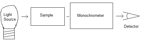
A schematic diagram of a typical infrared absorption spectroscopy experiment is shown below. The light is produced at the source (typically an incandescent light bulb or a glowbar), passes through the sample where some of the light can be absorbed, and then the monochrometer (which is typically either a grating or an interferometer) which is used to distinguish between the various frequencies of light, and finally the light is detected by a detector. Plotting detected intensity as a function of frequency produces the spectrum.
Determining a Force Constant
Consider the experimentally determined we value for carbon monoxide (CO.) The spectrum shows a strong absorption at \(2143 \; cm ^{-1}\) due to CO. Using this value for \(\omega_ {e}\) (it is actually a little off due to anharmonicity), the force constant can be determined for the molecule.
\[\omega_{e} =\dfrac{1}{2\pi c} \sqrt{\dfrac{k}{\mu } }\nonumber \]
Using a value of \(1.14 \times 10 ^{-26}\) kg for the reduced mass of the molecule, the force constant is found to be 1856 N/m. The literature value for this force constant is \(1860 \; cm ^{-1}\). Given that this calculation did not treat anharmonicity, the agreement is pretty good!
Progressions in Electronic Spectra
Electronic transition in diatomic molecules which can be observed in the visible and ultraviolet regions of the spectrum can have a great deal of vibrational structure as the molecule is free to vibrate in both the upper and lower states. Figure \(\PageIndex{2}\) shows vibrational progressions in the emission spectrum of \(\ce{AlBr}\) near 2800 Å (Fleming & Mathews, 1996).
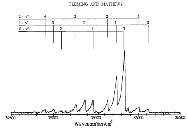
These progressions can be analyzed to provide dissociation energies for the electronic states involved in the transition.
If the vibrational energy function is truncated at the \(\omega_ {e} x _{e}\) level (as predicted by the Morse potential) the vibrational term value will reach a maximum value at some value of v. Any further vibrational excitation is predicted to lower the molecular energy. This is actually the dissociation limit. Therefore, the maximum value of \(v\) for a bound state (\(v_ {max}\) ) is the largest value of v for which the vibrational energy spacing is positive. The dissociation energy of the molecule is then given by the sum of vibrational energy spacings from \(v=0\) to \(v=v_ {max}\).
Determining a Dissociation Energy
To find the value of the dissociation energy, it is convenient to define the difference between successive vibrational terms as
\[\Delta G_{v+{\raise0.5ex\hbox{$\scriptstyle 1 $}\kern-0.1em/\kern-0.15em\lower0.25ex\hbox{$\scriptstyle 2 $}} } \equiv G_{v+1} -G_{v}\nonumber \]
Using the expression for \(G_ {v}\) as predicted by the Morse potential,
\[\begin{aligned} \Delta G_{v+1 / 2}= & \omega_e(v+3 / 2)-\omega_e x_e(v+3 / 2)^2-\omega_e(v+1 / 2)-\omega_e x_e(v+1 / 2)^2 \\[4pt] & =\omega_e(v+3 / 2-v-1 / 2)-\omega_e x_e\left(v^2+3 v+9 / 4-v^2-v-1 / 4\right) \\[4pt]&=\omega_e-\omega_e x_e(2 v+2) \\[4pt]&=\omega_e-2 \omega_e x_e(v+1)\end{aligned} \]
This suggests that a set of values of \(\Delta G_ {v+1/2}\) vs. \((v+1)\) should yield a straight line with a slope equal to -2\(\omega_ {e}\) \(x_ {e}\) and an intercept equal to \(\omega_ {e}\). And \(v_ {max}\) is determined by setting \(\Delta G_ {v+\frac{1}{2}}\) to zero and solving for \(v\) (Figure \(\PageIndex{3}\)).
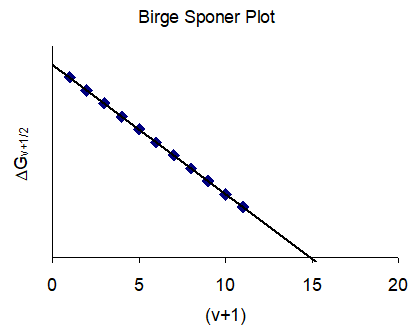
The Birge-Sponer method (Gaydon, 1946) can be used to determine the sum of vibrational spacings, and thus the dissociation of a molecule. The method involves plotting \(\Delta G_ {v+\frac{1}{2}}\) vs. \((v+1)\). The dissociation energy is taken as the area under the curve.
Vibrations of Polyatomic Molecules
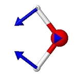
Nonlinear molecules have \(3N-6\) vibrational degrees of freedom, where N is the number of atoms in the molecule. Thus, a triatomic molecule such as water has three vibrational degrees of freedom. These account for the three vibrational modes of water (symmetric stretch, bend and antisymmetric stretch.)


Each mode will have a characteristic frequency. If each mode is treated as a harmonic oscillator, the total vibrational energy is given by
\[G=\sum _{i=1}^{3N-6}\omega _{i} (v_{i} +{\raise0.5ex\hbox{$\scriptstyle 1 $}\kern-0.1em/\kern-0.15em\lower0.25ex\hbox{$\scriptstyle 2 $}} )\nonumber \]
where \(\omega_ {i}\) is the frequency of the \(i ^{th}\) vibrational mode, and \(v_ {i}\) is the quantum number indicating the number of quanta of the \(i ^{th}\) mode excited. If anharmonicity is to be included, the expression becomes
\[G=\sum _{i=1}^{3N-6}\omega _{i} (v_{i} +{\raise0.5ex\hbox{$\scriptstyle 1 $}\kern-0.1em/\kern-0.15em\lower0.25ex\hbox{$\scriptstyle 2 $}} ) -\sum _{i=1}^{3N-6}\sum _{j=1}^{3N-6}x_{ij} \left(v_{i} +{\raise0.5ex\hbox{$\scriptstyle 1 $}\kern-0.1em/\kern-0.15em\lower0.25ex\hbox{$\scriptstyle 2 $}} \right)\left(v_{j} +{\raise0.5ex\hbox{$\scriptstyle 1 $}\kern-0.1em/\kern-0.15em\lower0.25ex\hbox{$\scriptstyle 2 $}} \right)\nonumber \]
where \(x_ {ij}\) is the anharmonicity term that couples the vibrational modes.