2.5: Superposition and Completeness

As stated previously, a system need not be in a state that is described by a single eigenfunction of the Hamiltonian. A system can be prepared such that any well-behaved, single valued, smooth function that vanishes at endpoints. When the wavefunction is not an eigenfunction of the Hamiltonian, the Superposition Principle can be used to greatly simplify how we work with the wave function. This is true because the so-called normal solutions \(\left(\psi_{n}(x)\right)\) to the Schrödinger Equation

\[\widehat{H} \psi_{n}(x)=E_{n} \psi_{n}(x)\nonumber \]

using the language of linear algebra, span the space of well-behaved functions that can describe the physics of the particle. That means that any arbitrary function that is 1) continuous, and 2) obeys the boundary conditions, can be expressed as a linear combination of these normal solutions:

\[\Phi(x)=\sum_{n} c_{n} \psi_{n}(x)\nonumber \]

where the coefficients \(c_{n}\) are calculated using the Fourier Transform shown below.

\[c_{n}=\int_{-\infty}^{\infty} \Phi(x) \psi_{n}(x) d x\nonumber \]

Superposition

This description also has a number of other important ramifications. Consider a particle in a box system prepared so that the wavefunction is given by

\[\Psi(x)=\dfrac{1}{\sqrt{2}} \psi_{1}(x)+\dfrac{1}{\sqrt{2}} \psi_{2}(x)\nonumber \]

where

\[\psi_{n}(x)=\sqrt{\dfrac{2}{a}} \sin \left(\dfrac{n \pi x}{a}\right)\nonumber \]

The first question one might ask is, "Is the wavefunction \(\Psi(\mathrm{x})\) normalized?" Well, let’s see!

\[\begin{aligned} \int_{0}^{a}(\Psi(x))^{2} d x &=\int_{0}^{a}\left[\left(\dfrac{1}{\sqrt{2}}\right) \psi_{1}+\left(\dfrac{1}{\sqrt{2}}\right) \psi_{2}\right]^{2} d x \\ &=\int_{0}^{a}\left(\dfrac{1}{2} \psi_{1} \psi_{1}+\psi_{1} \psi_{2}+\dfrac{1}{2} \psi_{2} \psi_{2}\right) d x \\ &=\dfrac{1}{2} \int_{0}^{a} \psi_{1} \psi_{1} d x+\int_{0}^{a} \psi_{1} \psi_{2} d x+\dfrac{1}{2} \int_{0}^{a} \psi_{2} \psi_{2} d x \\ &=\dfrac{1}{2}(1)+(0)+\dfrac{1}{2}(1) \\ &=1 \end{aligned}\nonumber \]

(Notice how the property \(\int \psi_{i} \psi_{j} d \tau=\delta_{i j}\) has been used to simplify the problem, by making the integral of the cross product in the middle vanish, and the integrals of the first and third terms go to unity.) So the wavefunction is normalized. Now, let’s evaluate the expectation value of energy \(\langle \mathrm{E} \rangle\).

\[\begin{aligned} \langle E\rangle &=\int_{0}^{a} \Psi \hat{H} \Psi d x \\ &=\int_{0}^{a}\left(\dfrac{1}{\sqrt{2}} \psi_{1}+\dfrac{1}{\sqrt{2}} \psi_{2}\right) \hat{H}\left(\dfrac{1}{\sqrt{2}} \psi_{1}+\dfrac{1}{\sqrt{2}} \psi_{2}\right) d x \\ &=\int_{0}^{a}\left(\dfrac{1}{\sqrt{2}} \psi_{1}+\dfrac{1}{\sqrt{2}} \psi_{2}\right)\left(\dfrac{E_{1}}{\sqrt{2}} \psi_{1}+\dfrac{E_{2}}{\sqrt{2}} \psi_{2}\right) d x \\ &=\int_{0}^{a}\left(\dfrac{E_{1}}{2} \psi_{1} \psi_{1}+\dfrac{E_{1}}{2} \psi_{2} \psi_{1}+\dfrac{E_{2}}{2} \psi_{1} \psi_{2}+\dfrac{E_{2}}{2} \psi_{2} \psi_{2}\right) d x \\ &=\dfrac{E_{1}}{2} \int_{0}^{a} \psi_{1} \psi_{1} d x+\dfrac{E_{1}}{2} \int_{0}^{a} \psi_{2} \psi_{1} d x+\dfrac{E_{2}}{2} \int_{0}^{a} \psi_{1} \psi_{2} d x \dfrac{E_{2}}{2} \int_{0}^{a} \psi_{2} \psi_{2} d x \\ &=\dfrac{E_{1}}{2}+0+0+\dfrac{E_{2}}{2} \end{aligned}\nonumber \]

So the expectation value is given by the average of \(E_{1}\) and \(E_{2}\). This result is only possible if half of the time the energy is measured, the observed value is \(\mathrm{E}_{1}\) and the other half \(\mathrm{E}_{2}\). In other words, the probability of measuring \(E_{1}\) is \(\frac{1}{2}\) and that of \(E_{2}\) is \(\frac{1}{2}\). It is also important to note that these probabilities are given by the Fourier coefficients of

\[c_{1}=1 / \sqrt{2}, c_{2}=1 / \sqrt{2} \text { and } c_{n}=0 \text { for all other } n\nonumber \]

It can be concluded that the probability of measuring \(E_{n}\) is given by \(\left|c_{n}{ }^{2}\right|\).

\[P\left(E_{n}\right)=\left|c_{n}^{2}\right|\nonumber \]

Completeness

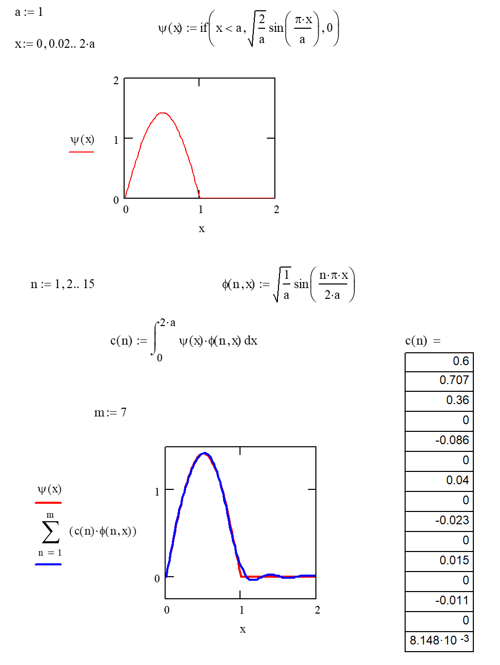
Imagine the following scenario. A quantum mechanical particle of mass \(m\) in a onedimensional box of length \(a\) is prepared such that its wavefunction is given by \(\psi_{1}(\mathrm{x})\). Instantaneously, the length of the box increases to \(2 a\). The particle is no longer in an eigenstate of the new system. Rather, its wavefunction will look like the function depicted below in the MatchCad worksheet.

The function can be described as a superposition of wavefunctions that are eigenfunctions of the Hamiltonian that reflects the new length of the box. A MathCad worksheet that reflects this expansion is given on the next page. The larger the value of \(\mathrm{m}\) selected, the better the representation of the wavefunction.

Figure \(\PageIndex{1}\)

The above problem is analogous to what happens when an atom undergoes radioactive decay by something such as \(\beta\)-particle emission from the nucleus. In that case, the nuclear charge suddenly changes (changing the potential energy function and thus the Hamiltonian.) The change happens effectively instantaneously compared to the time required for the atom to react. The atom suddenly finds itself in a non-eigenstate, the nature of which will govern how the atom changes in time to respond to the nuclear decay. The superposition of eigenfunctions of the new Hamiltonian will give a description of the atom immediately following the decay, and the overall wavefunction will evolve in time based on how it is predicted to do so according to the fifth postulate.

The superposition theorem allows for a complete description of a wavefunction according to the needs to the quantum theory - even if the wavefunction being described by a superposition of states is not an eigenfunction of the Hamiltonian! (Now how much would you pay?)