2.3: The One-Dimensional Particle in a Box

Imagine a particle of mass \(m\) constrained to travel back and forth in a one dimensional box of length \(a\). For convenience, we define the endpoints of the box to be located at \(\mathrm{x}=0\) and \(\mathrm{x}\) \(=a\). The derivation of wavefunctions and energy levels and the properties of the system using the tools of quantum mechanics will be instructive as we move forward in our studies of quantum mechanics.

The Hamiltonian

Whenever we begin a new quantum mechanical problem, the first challenge is to write the Hamiltonian that describes the system. This always has two parts - a Kinetic Energy term (which is always the same for each particle) and a Potential Energy term (that is different for each new system.)

The kinetic energy term in one dimension for a single particle is always given by

\[\hat{T}=-\dfrac{\hbar^{2}}{2 m} \dfrac{d^{2}}{d x^{2}}\nonumber\]

This operator can be derived from the momentum operator based on the relationship between momentum and kinetic energy that comes from classical physics. Namely

\[T=\dfrac{p^{2}}{2 m}\nonumber\]

As such,

\[\begin{aligned} &\hat{T}=\dfrac{p^{2}}{2 m} \\ &=\dfrac{1}{2 m}\left(-i \hbar \dfrac{d}{d x}\right) \\ &=\dfrac{(-i \hbar)^{2}}{2 m} \dfrac{d^{2}}{d x^{2}} \\ &=-\dfrac{\hbar^{2}}{2 m} \dfrac{d^{2}}{d x^{2}} \end{aligned}\nonumber\]

The potential energy function is also fairly simple for this problem. The potential energy is infinite outside of the box \((\mathrm{x}<0\) and \(\mathrm{x}>\mathrm{a})\) and zero every place else. This forces the particle to be in the box at all times. It also limits the relevant space of the problem to lie between \(\mathrm{x}=0\) and \(\mathrm{x}=\) \(a\) since the infinite potential energy precludes the particle from ever existing outside of the limits of \(\mathrm{x}=0\) and \(\mathrm{x}=a\).

\[U(x)=\mid \begin{array}{lll} \infty & \text { if } & x<0 \\ 0 & \text { if } & 0 \leq x \leq a \\ \infty & \text { if } & x>a \end{array}\nonumber\]

Figure \(\PageIndex{1}\)

So for the problem, limited to the space inside the box, the Hamiltonian can be written

\[\hat{H}=-\dfrac{\hbar^{2}}{2 m} \dfrac{d^{2}}{d x^{2}}\nonumber\]

And the Schrödinger equation can be written as

\[-\dfrac{\hbar^{2}}{2 m} \dfrac{d^{2}}{d x^{2}} \psi(x)=E \psi(x)\nonumber\]

where \(\psi(\mathrm{x})\) is the wavefunction describing the state of the particle. There are a number of approaches that can be used to solve this equation to find the wavefunctions \(\psi(\mathrm{x})\) which satisfy the differential equation.

The Solution

We will solve this problem two different ways. First, we will solve it using the de Broglie wavelength (an algebraic solution) and then using the Schrödinger equation (an eigenvalue/eigenfunction approach.)

The de Broglie Approach

Before trying to solve the problem using Schrödinger’s equation, let’s use the de Broglie condition to solve the problem algebraically. Recall that de Broglie suggested that a particle can be treated as a wave, the wavelength of which is given by \(\lambda=\mathrm{h} / \mathrm{p}\), where \(\mathrm{h}\) is Planck’s constant, and \(p\) is the momentum of the particle.

The necessary conditions on the de Broglie wave are that the wave itself must vanish at the ends of the box (in order to satisfy the first postulate, since the particle can never escape the box.) This will happen for very specific wavelengths which are dependent on the length of the box itself. This is very common in physics for any system with a wave nature. When the wave is constrained to a specific geometry, the system will "ring" with frequencies (and thus wavelengths) characteristic of the medium and the geometry. Quantum mechanical systems are no different in that regard.

Figure \(\PageIndex{2}\)

What will be required in order to create a standing wave is that the length of the box \((a)\) must be an integral multiple of half de Broglie wavelengths \((\lambda / 2)\).

\[a=n \dfrac{\lambda}{2}\nonumber\]

Given that the de Broglie wavelength is related to momentum, it is simple to derive the following relationship, indicating the possible values for momentum.

\[\begin{aligned} a &=n \dfrac{\lambda}{2} \\ &=\dfrac{n h}{2 p} \\ p &=\dfrac{n h}{2 a} \end{aligned}\nonumber\]

Given the relationship between momentum and kinetic energy, the expected expression for energy levels can be derived.

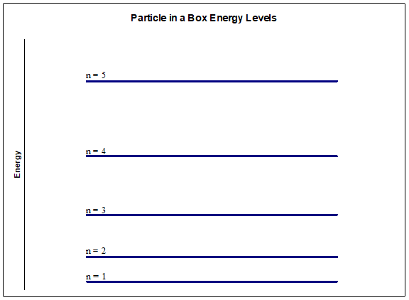
\[E=\dfrac{p^{2}}{2 m}=\dfrac{1}{2 m}\left(\dfrac{n h}{2 a}\right)^{2}=\dfrac{n^{2} h^{2}}{8 m a^{2}}\nonumber\]

And since the energy depends on \(n^{2}\), the spacings between successive energy levels increases as the energy increases.

Figure \(\PageIndex{3}\)

Now let’s see if we can derive this expression based on the Schrödinger equation.

The Schrödinger equation: the wavefunctions

The time-independent Schrödinger equation can be written

\[\hat{H} \psi=E \psi\nonumber\]

Where \(H\) is the Hamiltonian operator that was derived in section B.2, \(\psi\) is the wavefunction describing the system, and \(E\), the eigenvalue of the Hamiltonian, gives the energy. The wavefunctions are derived so that they are eigenfunctions of the Hamiltonian operator. Substituting the specific statement of the Hamiltonian

\[-\dfrac{\hbar^{2}}{2 m} \dfrac{d^{2}}{d x^{2}} \psi=E \psi\nonumber\]

For convenience, we can gather all of the constants in one place by making a substitution

\[-k^{2}=-\dfrac{2 m E}{\hbar^{2}}\nonumber\]

The particular choice if the form of this substitution is made to simplify the solutions by avoiding (for now) imaginary functions. With the substitution, the Schrödinger equation can be rewritten as

\[\dfrac{d^{2}}{d x^{2}} \psi=-k^{2} \psi\nonumber\]

As was the case for the classical wave-on-a-string problem, this is a second order ordinary differential equation, and this has two linearly independent solutions. A general solution is given by a linear combination of two linearly independent solutions, so one way to write a solution is

\[\psi=A \sin (k x)+B \cos (k x)\nonumber\]

Now we can focus on evaluating \(\mathrm{A}, \mathrm{B}\) and \(\mathrm{k}\) based on the boundary conditions. The boundary conditions are that the wavefunction must go to 0 at the ends of the box, in accordance with the first postulate.

The first boundary condition, \(\psi(0)=0\), yields the following result:

\[\begin{aligned} \psi(0) &=A \sin (k \cdot 0)+B \cos (k \cdot 0) \\ &=0+B=0 \end{aligned}\nonumber\]

So \(\mathrm{B}=0\) and the cosine term must vanish. Focusing only on what has not vanished from the solutions, the second boundary condition, \(\psi(a)=0\), can be applied.

\[\psi(a)=A \sin (k \cdot a)=0\nonumber\]

There are two trivial ways to make this true. One is to make \(\mathrm{A}=0\) and the other is to make \(\mathrm{k}=\) 0 . Both are trivial solutions and unimportant (but fun to mention in class!) The other way to force the function to 0 at \(\mathrm{x}=\mathrm{a}\) is to insure that the sine function is zero by forcing

\[k \cdot a=n \pi\nonumber\]

where \(\mathrm{n}\) is an integer \((\mathrm{n}=1,2,3 \ldots)\), since the sine function crosses zero every \(\mathrm{n} \pi\) radians. This is an important point: the application of a boundary condition leads to the introduction of a quantum number and fixed the results to only functions where that number has a value taken from a very specific list. In fact, the origin of quantum numbers in all problems is the result of the application of boundary conditions.

Solving for \(\mathrm{k}\) and substituting yields

\[\psi(x)=A \sin \left(\dfrac{n \pi x}{a}\right)\nonumber\]

This is as far as the boundary conditions can get us. The value of \(\mathrm{A}\) is determined based on the first postulate of quantum mechanics, which says that the square of the wavefunction must give a probability distribution as to where the particle can be measured to be. Since all measurements must place the particle in the box, the sum of probabilities at all of the possible locations in the box must equal unity. This implies the condition that

\[\int_{0}^{a}(\psi(x))^{2} d x=1\nonumber\]

Solving for A yields

\[\begin{aligned} \int_{0}^{a}(\psi(x))^{2} d x &=A^{2} \int_{0}^{a} \sin ^{2}\left(\dfrac{n \pi x}{a}\right) d x \\ &=A^{2}\left[\dfrac{x}{2}-\dfrac{\sin \left(\dfrac{2 n \pi x}{a}\right)}{\left(\dfrac{4 n \pi}{a}\right)}\right]_{0}^{a} \\ &=A^{2}\left(\dfrac{a}{2}-0-0+0\right) \\ A &=\sqrt{\dfrac{2}{a}} \end{aligned}\nonumber\]

Notice that the value of A did not depend on the quantum number n. Normalization constants usually do have some dependence on the quantum numbers that arise from the application of boundary conditions, but this is one of the rare problems in which the normalization constant does not.

The Schrödinger Equation: the energy levels

Whenever we solve a quantum mechanical problem, there are two important things at which we must look: the energy levels and the wavefunctions. To chemists, the energy levels are the most important part, as the energy levels govern the chemistry the system can do. To a physicist, it is the wavefunctions that are important as they contain all of the information about the physical nature of the system.

The energy levels can be derived using the normalized wavefunctions and the Schrödinger equation.

\[\begin{aligned} \hat{H} \psi &=E \psi \\[4pt] \underbrace{-\dfrac{\hbar^{2}}{2 m} \dfrac{d^{2}}{d x^{2}}}_{\hat{H}} \underbrace{\sqrt{\dfrac{2}{a}} \sin \left(\dfrac{n \pi x}{a}\right)}_{\psi} &= \underbrace{\dfrac{\hbar^{2}}{2 m}\left(\dfrac{n \pi}{a}\right)^{2}}_{E} \underbrace{\sqrt{\dfrac{2}{a}} \sin \left(\dfrac{n \pi x}{a}\right)}_{\psi} \end{aligned}\]

Comparison (or solving for \(E\)) yields the following

\[E=\dfrac{n^{2} \pi^{2} \hbar^{2}}{2 m a^{2}}\nonumber\]

which looks similar to, but not exactly like the result produced using the de Broglie relationship. In fact, it is the identical result! Making the substitution \(\hbar=h / 2 \pi\), it is easy to show that

\[E=\dfrac{n^{2} h^{2}}{8 m a^{2}}\nonumber\]

These energy levels depend on \(\mathrm{n}^{2}\), and so doubling the quantum number \(\mathrm{n}\) quadruples the energy. Another way of saying this is that the energy level spacings (the difference in energy between two successive levels) increase with increasing \(\mathrm{n}\) or energy.

It is also interesting to note that the energy levels are given by a real (non-imaginary) expression. This is to be expected since the energy is the eigenvalue of a Hermitian operator, the Hamiltonian, and thus must be a real value.

Properties of the Wavefunctions

The wavefunctions for the one-dimensional particle in a box problem are given by

\[\psi_{n}(x)=\sqrt{\dfrac{2}{a}} \sin \left(\dfrac{n \pi x}{a}\right)\nonumber\]

These wavefunctions have many important properties.

Orthogonality

Similar to the relationship of Hermitian operators having real eigenvalues, the eigenfunctions of Hermitian operators must be orthogonal. Our wavefunctions are actually an infinite set of function, any pair of which must cause the inner product integral to vanish. Mathematically, this looks like

\[\int_{0}^{a} \psi_{n}(x) \cdot \psi_{m}(x) d x=0 \quad n \neq m\nonumber\]

This relationship is easy to verify. To do so, we will make use of the following result taken from a standard table of integrals.

\[\int \sin (\alpha x) \sin (\beta x) d x=\dfrac{\sin [(\alpha-\beta) x]}{2(\alpha-\beta)}-\dfrac{\sin [(\alpha+\beta) x]}{2(\alpha+\beta)} \quad \alpha \neq \beta\nonumber\]

Noting that \(\alpha=\dfrac{n \pi}{a}\) and \(\beta=\dfrac{m \pi}{a}\), substitution into the above relationship yields

\[\begin{aligned} \int_{0}^{a} \psi_{n}(x) \cdot \psi_{m}(x) d x &=\left[\dfrac{\sin \left[\dfrac{\pi}{a}(n-m) x\right]}{2\left(\dfrac{\pi}{a}(n-m)\right)}-\dfrac{\sin \left[\dfrac{\pi}{a}(n+m) x\right]}{2\left(\dfrac{\pi}{a}(n+m)\right)}\right]_{0}^{a} \\ &=\left[\dfrac{\sin [\pi(n-m)]}{2\left(\dfrac{\pi}{a}(n-m)\right)}-\dfrac{\sin [\pi(n+m)]}{2\left(\dfrac{\pi}{a}(n+m)\right)}-0+0\right] \end{aligned}\nonumber\]

And since \(n\) and \(m\) are integer, \(n-m\) and \(n+m\) must also be integers. And the sine of an integral multiple of \(\pi\) is always zero, it is easy to show that this function vanishes for any \(n \neq m\).

Normalization

When \(n=m\) the integral becomes

\[\int_{0}^{a}\left[\psi_{n}(x)\right]^{2} d x=\dfrac{2}{a} \int_{0}^{a} \sin ^{2}\left(\dfrac{n \pi x}{a}\right) d x\nonumber\]

which can be evaluated using the result from a table of integrals

\[\int \sin ^{2}(\alpha x) d x=\dfrac{x}{2}-\dfrac{\sin (2 \alpha x)}{4 \alpha}\nonumber\]

So making the substitution \(\alpha=\dfrac{n \pi}{a}\)

\[\begin{aligned} &\dfrac{2}{a} \int_{0}^{a} \sin ^{2}\left(\dfrac{n \pi x}{a}\right) d x=\dfrac{2}{a}\left[\dfrac{x}{2}-\dfrac{\sin \left(\dfrac{2 n \pi x}{a}\right)}{4(n \pi / a)}\right]_{0}^{a} \\ &=\dfrac{2}{a}\left[\dfrac{a}{2}-0-0+0\right] \\ &=1 \end{aligned}\nonumber\]

This result shouldn’t be surprising since the value \(\mathrm{A}=\sqrt{\dfrac{2}{a}}\) was chosen to ensure the result! Specifically, it was chosen so as to normalize the wave functions.

Example \(\PageIndex{1}\)

Show that the wavefunction

\[\Psi(x)=\sqrt{\dfrac{30}{a^{5}}} \cdot x(a-x)\nonumber\]

is normalized for a particle in a box of length \(a\).

Solution

The wavefunction is normalized if

\[\int_{0}^{a} \Psi(x) \Psi(x) d x=1\nonumber\]

This can be demonstrated by plugging the wavefunction into the relationship and testing to see if it is true:

\[\begin{aligned} \int_{0}^{a} \sqrt{\dfrac{30}{a^{5}}} \cdot x(a-x) & \sqrt{\dfrac{30}{a^{5}}} \cdot x(a-x) d x=\dfrac{30}{a^{5}} \int_{0}^{a} x^{2}\left(a^{2}-2 a x+x^{2}\right) d x \\ &=\dfrac{30}{a^{5}} \int_{0}^{a}\left(a^{2} x^{2}-2 a x^{3}+x^{4}\right) d x \\ &=\dfrac{30}{a^{5}}\left[\dfrac{a^{2} x^{3}}{3}-\dfrac{2 a x^{4}}{4}+\dfrac{x^{5}}{5}\right]_{0}^{a} \\ &=\dfrac{30}{a^{5}}\left(\dfrac{a^{5}}{3}-\dfrac{a^{5}}{2}+\dfrac{a^{5}}{5}-0+0-0\right) \\ &=\dfrac{30}{a^{5}}\left(\dfrac{10 a^{5}}{30}-\dfrac{15 a^{5}}{30}+\dfrac{6 a^{5}}{30}\right) \\ &=\dfrac{30}{a^5}\left(\dfrac{a^5}{30}\right) \\ &=1 \end{aligned}\]

Therefore the wavefunction is normalized!