
32.9: Series and Limits
- Page ID
- 38832
\( \newcommand{\vecs}[1]{\overset { \scriptstyle \rightharpoonup} {\mathbf{#1}} } \)
\( \newcommand{\vecd}[1]{\overset{-\!-\!\rightharpoonup}{\vphantom{a}\smash {#1}}} \)
\( \newcommand{\id}{\mathrm{id}}\) \( \newcommand{\Span}{\mathrm{span}}\)
( \newcommand{\kernel}{\mathrm{null}\,}\) \( \newcommand{\range}{\mathrm{range}\,}\)
\( \newcommand{\RealPart}{\mathrm{Re}}\) \( \newcommand{\ImaginaryPart}{\mathrm{Im}}\)
\( \newcommand{\Argument}{\mathrm{Arg}}\) \( \newcommand{\norm}[1]{\| #1 \|}\)
\( \newcommand{\inner}[2]{\langle #1, #2 \rangle}\)
\( \newcommand{\Span}{\mathrm{span}}\)
\( \newcommand{\id}{\mathrm{id}}\)
\( \newcommand{\Span}{\mathrm{span}}\)
\( \newcommand{\kernel}{\mathrm{null}\,}\)
\( \newcommand{\range}{\mathrm{range}\,}\)
\( \newcommand{\RealPart}{\mathrm{Re}}\)
\( \newcommand{\ImaginaryPart}{\mathrm{Im}}\)
\( \newcommand{\Argument}{\mathrm{Arg}}\)
\( \newcommand{\norm}[1]{\| #1 \|}\)
\( \newcommand{\inner}[2]{\langle #1, #2 \rangle}\)
\( \newcommand{\Span}{\mathrm{span}}\) \( \newcommand{\AA}{\unicode[.8,0]{x212B}}\)
\( \newcommand{\vectorA}[1]{\vec{#1}} % arrow\)
\( \newcommand{\vectorAt}[1]{\vec{\text{#1}}} % arrow\)
\( \newcommand{\vectorB}[1]{\overset { \scriptstyle \rightharpoonup} {\mathbf{#1}} } \)
\( \newcommand{\vectorC}[1]{\textbf{#1}} \)
\( \newcommand{\vectorD}[1]{\overrightarrow{#1}} \)
\( \newcommand{\vectorDt}[1]{\overrightarrow{\text{#1}}} \)
\( \newcommand{\vectE}[1]{\overset{-\!-\!\rightharpoonup}{\vphantom{a}\smash{\mathbf {#1}}}} \)
\( \newcommand{\vecs}[1]{\overset { \scriptstyle \rightharpoonup} {\mathbf{#1}} } \)
\( \newcommand{\vecd}[1]{\overset{-\!-\!\rightharpoonup}{\vphantom{a}\smash {#1}}} \)
\(\newcommand{\avec}{\mathbf a}\) \(\newcommand{\bvec}{\mathbf b}\) \(\newcommand{\cvec}{\mathbf c}\) \(\newcommand{\dvec}{\mathbf d}\) \(\newcommand{\dtil}{\widetilde{\mathbf d}}\) \(\newcommand{\evec}{\mathbf e}\) \(\newcommand{\fvec}{\mathbf f}\) \(\newcommand{\nvec}{\mathbf n}\) \(\newcommand{\pvec}{\mathbf p}\) \(\newcommand{\qvec}{\mathbf q}\) \(\newcommand{\svec}{\mathbf s}\) \(\newcommand{\tvec}{\mathbf t}\) \(\newcommand{\uvec}{\mathbf u}\) \(\newcommand{\vvec}{\mathbf v}\) \(\newcommand{\wvec}{\mathbf w}\) \(\newcommand{\xvec}{\mathbf x}\) \(\newcommand{\yvec}{\mathbf y}\) \(\newcommand{\zvec}{\mathbf z}\) \(\newcommand{\rvec}{\mathbf r}\) \(\newcommand{\mvec}{\mathbf m}\) \(\newcommand{\zerovec}{\mathbf 0}\) \(\newcommand{\onevec}{\mathbf 1}\) \(\newcommand{\real}{\mathbb R}\) \(\newcommand{\twovec}[2]{\left[\begin{array}{r}#1 \\ #2 \end{array}\right]}\) \(\newcommand{\ctwovec}[2]{\left[\begin{array}{c}#1 \\ #2 \end{array}\right]}\) \(\newcommand{\threevec}[3]{\left[\begin{array}{r}#1 \\ #2 \\ #3 \end{array}\right]}\) \(\newcommand{\cthreevec}[3]{\left[\begin{array}{c}#1 \\ #2 \\ #3 \end{array}\right]}\) \(\newcommand{\fourvec}[4]{\left[\begin{array}{r}#1 \\ #2 \\ #3 \\ #4 \end{array}\right]}\) \(\newcommand{\cfourvec}[4]{\left[\begin{array}{c}#1 \\ #2 \\ #3 \\ #4 \end{array}\right]}\) \(\newcommand{\fivevec}[5]{\left[\begin{array}{r}#1 \\ #2 \\ #3 \\ #4 \\ #5 \\ \end{array}\right]}\) \(\newcommand{\cfivevec}[5]{\left[\begin{array}{c}#1 \\ #2 \\ #3 \\ #4 \\ #5 \\ \end{array}\right]}\) \(\newcommand{\mattwo}[4]{\left[\begin{array}{rr}#1 \amp #2 \\ #3 \amp #4 \\ \end{array}\right]}\) \(\newcommand{\laspan}[1]{\text{Span}\{#1\}}\) \(\newcommand{\bcal}{\cal B}\) \(\newcommand{\ccal}{\cal C}\) \(\newcommand{\scal}{\cal S}\) \(\newcommand{\wcal}{\cal W}\) \(\newcommand{\ecal}{\cal E}\) \(\newcommand{\coords}[2]{\left\{#1\right\}_{#2}}\) \(\newcommand{\gray}[1]{\color{gray}{#1}}\) \(\newcommand{\lgray}[1]{\color{lightgray}{#1}}\) \(\newcommand{\rank}{\operatorname{rank}}\) \(\newcommand{\row}{\text{Row}}\) \(\newcommand{\col}{\text{Col}}\) \(\renewcommand{\row}{\text{Row}}\) \(\newcommand{\nul}{\text{Nul}}\) \(\newcommand{\var}{\text{Var}}\) \(\newcommand{\corr}{\text{corr}}\) \(\newcommand{\len}[1]{\left|#1\right|}\) \(\newcommand{\bbar}{\overline{\bvec}}\) \(\newcommand{\bhat}{\widehat{\bvec}}\) \(\newcommand{\bperp}{\bvec^\perp}\) \(\newcommand{\xhat}{\widehat{\xvec}}\) \(\newcommand{\vhat}{\widehat{\vvec}}\) \(\newcommand{\uhat}{\widehat{\uvec}}\) \(\newcommand{\what}{\widehat{\wvec}}\) \(\newcommand{\Sighat}{\widehat{\Sigma}}\) \(\newcommand{\lt}{<}\) \(\newcommand{\gt}{>}\) \(\newcommand{\amp}{&}\) \(\definecolor{fillinmathshade}{gray}{0.9}\)Maclaurin Series
A function \(f(x)\) can be expressed as a series in powers of \(x\) as long as \(f(x)\) and all its derivatives are finite at \(x=0\). For example, we will prove shortly that the function \(f(x) = \dfrac{1}{1-x}\) can be expressed as the following infinite sum:
\[\label{eq1}\dfrac{1}{1-x}=1+x+x^2+x^3+x^4 + \ldots \]
We can write this statement in this more elegant way:
\[\label{eq2}\dfrac{1}{1-x}=\displaystyle\sum_{n=0}^{\infty} x^{n} \]
If you are not familiar with this notation, the right side of the equation reads “sum from \(n=0\) to \(n=\infty\) of \(x^n.\)” When \(n=0\), \(x^n = 1\), when \(n=1\), \(x^n = x\), when \(n=2\), \(x^n = x^2\), etc (compare with Equation \ref{eq1}). The term “series in powers of \(x\)” means a sum in which each summand is a power of the variable \(x\). Note that the number 1 is a power of \(x\) as well (\(x^0=1\)). Also, note that both Equations \ref{eq1} and \ref{eq2} are exact, they are not approximations.
Similarly, we will see shortly that the function \(e^x\) can be expressed as another infinite sum in powers of \(x\) (i.e. a Maclaurin series) as:
\[\label{expfunction}e^x=1+x+\dfrac{1}{2} x^2+\dfrac{1}{6}x^3+\dfrac{1}{24}x^4 + \ldots \]
Or, more elegantly:
\[\label{expfunction2}e^x=\displaystyle\sum_{n=0}^{\infty}\dfrac{1}{n!} x^{n} \]
where \(n!\) is read “n factorial” and represents the product \(1\times 2\times 3...\times n\). If you are not familiar with factorials, be sure you understand why \(4! = 24\). Also, remember that by definition \(0! = 1\), not zero.
At this point you should have two questions: 1) how do I construct the Maclaurin series of a given function, and 2) why on earth would I want to do this if \(\dfrac{1}{1-x}\) and \(e^x\) are fine-looking functions as they are. The answer to the first question is easy, and although you should know this from your calculus classes we will review it again in a moment. The answer to the second question is trickier, and it is what most students find confusing about this topic. We will discuss different examples that aim to show a variety of situations in which expressing functions in this way is helpful.
How to obtain the Maclaurin Series of a Function
In general, a well-behaved function (\(f(x)\) and all its derivatives are finite at \(x=0\)) will be expressed as an infinite sum of powers of \(x\) like this:
\[\label{eq3}f(x)=\displaystyle\sum_{n=0}^{\infty}a_n x^{n}=a_0+a_1 x + a_2 x^2 + \ldots + a_n x^n \]
Be sure you understand why the two expressions in Equation \ref{eq3} are identical ways of expressing an infinite sum. The terms \(a_n\) are called the coefficients, and are constants (that is, they are NOT functions of \(x\)). If you end up with the variable \(x\) in one of your coefficients go back and check what you did wrong! For example, in the case of \(e^x\) (Equation \ref{expfunction}), \(a_0 =1, a_1=1, a_2 = 1/2, a_3=1/6, etc\). In the example of Equation \ref{eq1}, all the coefficients equal 1. We just saw that two very different functions can be expressed using the same set of functions (the powers of \(x\)). What makes \(\dfrac{1}{1-x}\) different from \(e^x\) are the coefficients \(a_n\). As we will see shortly, the coefficients can be negative, positive, or zero.
How do we calculate the coefficients? Each coefficient is calculated as:
\[\label{series:coefficients}a_n=\dfrac{1}{n!} \left( \dfrac{d^n f(x)}{dx^n} \right)_0 \]
That is, the \(n\)-th coefficient equals one over the factorial of \(n\) multiplied by the \(n\)-th derivative of the function \(f(x)\) evaluated at zero. For example, if we want to calculate \(a_2\) for the function \(f(x)=\dfrac{1}{1-x}\), we need to get the second derivative of \(f(x)\), evaluate it at \(x=0\), and divide the result by \(2!\). Do it yourself and verify that \(a_2=1\). In the case of \(a_0\) we need the zeroth-order derivative, which equals the function itself (that is, \(a_0 = f(0)\), because \(\dfrac{1}{0!}=1\)). It is important to stress that although the derivatives are usually functions of \(x\), the coefficients are constants because they are expressed in terms of the derivatives evaluated at \(x=0\).
Note that in order to obtain a Maclaurin series we evaluate the function and its derivatives at \(x=0\). This procedure is also called the expansion of the function around (or about) zero. We can expand functions around other numbers, and these series are called Taylor series (see Section 3).
Obtain the Maclaurin series of \(sin(x)\).
Solution
We need to obtain all the coefficients (\(a_0, a_1...etc\)). Because there are infinitely many coefficients, we will calculate a few and we will find a general pattern to express the rest. We will need several derivatives of \(sin(x)\), so let’s make a table:
| \(n\) | \(\dfrac{d^n f(x)}{dx^n}\) | \(\left( \dfrac{d^n f(x)}{dx^n} \right)_0\) |
|---|---|---|
| 0 | \(\sin (x)\) | 0 |
| 1 | \(\cos (x)\) | 1 |
| 2 | \(-\sin (x)\) | 0 |
| 3 | \(-\cos (x)\) | -1 |
| 4 | \(\sin (x)\) | 0 |
| 5 | \(\cos (x)\) | 1 |
Remember that each coefficient equals \(\left( \dfrac{d^n f(x)}{dx^n} \right)_0\) divided by \(n!\), therefore:
| \(n\) | \(n!\) | \(a_n\) |
|---|---|---|
| 0 | 1 | 0 |
| 1 | 1 | 1 |
| 2 | 2 | 0 |
| 3 | \(6\) | \(-\dfrac{1}{6}\) |
| 4 | \(24\) | 0 |
| 5 | \(120\) | \(\dfrac{1}{120}\) |
This is enough information to see the pattern (you can go to higher values of \(n\) if you don’t see it yet):
- the coefficients for even values of \(n\) equal zero.
- the coefficients for \(n = 1, 5, 9, 13,...\) equal \(1/n!\)
- the coefficients for \(n = 3, 7, 11, 15,...\) equal \(-1/n!\).
Recall that the general expression for a Maclaurin series is \(a_0+a_1 x + a_2 x^2...a_n x^n\), and replace \(a_0...a_n\) by the coefficients we just found:
\[\displaystyle{\color{Maroon}\sin (x) = x - \dfrac{1}{3!} x^3+ \dfrac{1}{5!} x^5 -\dfrac{1}{7!} x^7...} \nonumber \]
This is a correct way of writing the series, but in the next example we will see how to write it more elegantly as a sum.
Express the Maclaurin series of \(\sin (x)\) as a sum.
Solution
In the previous example we found that:
\[\label{series:sin}\sin (x) = x - \dfrac{1}{3!} x^3+ \dfrac{1}{5!} x^5 -\dfrac{1}{7!} x^7... \]
We want to express this as a sum:
\[\displaystyle\sum_{n=0}^{\infty}a_n x^{n} \nonumber \]
The key here is to express the coefficients \(a_n\) in terms of \(n\). We just concluded that 1) the coefficients for even values of \(n\) equal zero, 2) the coefficients for \(n = 1, 5, 9, 13,...\) equal \(1/n!\) and 3) the coefficients for \(n = 3, 7, 11,...\) equal \(-1/n!\). How do we put all this information together in a unique expression? Here are three possible (and equally good) answers:
- \(\displaystyle{\color{Maroon}\sin (x)=\displaystyle\sum_{n=0}^{\infty} \left( -1 \right) ^n \dfrac{1}{(2n+1)!} x^{2n+1}}\)
- \(\displaystyle{\color{Maroon}\sin (x)=\displaystyle\sum_{n=1}^{\infty} \left( -1 \right) ^{(n+1)} \dfrac{1}{(2n-1)!} x^{2n-1}}\)
- \(\displaystyle{\color{Maroon}\sin (x)=\displaystyle\sum_{n=0}^{\infty} cos(n \pi) \dfrac{1}{(2n+1)!} x^{2n+1}}\)
This may look impossibly hard to figure out, but let me share a few tricks with you. First, we notice that the sign in Equation \ref{series:sin} alternates, starting with a “+”. A mathematical way of doing this is with a term \((-1)^n\) if your sum starts with \(n=0\), or \((-1)^{(n+1)}\) if you sum starts with \(n=1\). Note that \(\cos (n \pi)\) does the same trick.
| \(n\) | \((-1)^n\) | \((-1)^{n+1}\) | \(\cos (n \pi)\) |
|---|---|---|---|
| 0 | 1 | -1 | 1 |
| 1 | -1 | 1 | -1 |
| 2 | 1 | -1 | 1 |
| 3 | -1 | 1 | -1 |
We have the correct sign for each term, but we need to generate the numbers \(1, \dfrac{1}{3!}, \dfrac{1}{5!}, \dfrac{1}{7!},...\) Notice that the number “1” can be expressed as \(\dfrac{1}{1!}\). To do this, we introduce the second trick of the day: we will use the expression \(2n+1\) to generate odd numbers (if you start your sum with \(n=0\)) or \(2n-1\) (if you start at \(n=1\)). Therefore, the expression \(\dfrac{1}{(2n+1)!}\) gives \(1, \dfrac{1}{3!}, \dfrac{1}{5!}, \dfrac{1}{7!},...\), which is what we need in the first and third examples (when the sum starts at zero).
Lastly, we need to use only odd powers of \(x\). The expression \(x^{(2n+1)}\) generates the terms \(x, x^3, x^5...\) when you start at \(n=0\), and \(x^{(2n-1)}\) achieves the same when you start your series at \(n=1\).
Confused about writing sums using the sum operator \((\sum)\)? This video will help: http://tinyurl.com/lvwd36q
Need help? The links below contain solved examples.
External links:
Finding the maclaurin series of a function I: http://patrickjmt.com/taylor-and-maclaurin-series-example-1/
Finding the maclaurin series of a function II: http://www.youtube.com/watch?v= dp2ovDuWhro
Finding the maclaurin series of a function III: http://www.youtube.com/watch?v= WWe7pZjc4s8
Graphical Representation
From Equation \(\ref{eq3}\) and the examples we discussed above, it should be clear at this point that any function whose derivatives are finite at \(x=0\) can be expressed by using the same set of functions: the powers of \(x\). We will call these functions the basis set. A basis set is a collection of linearly independent functions that can represent other functions when used in a linear combination.
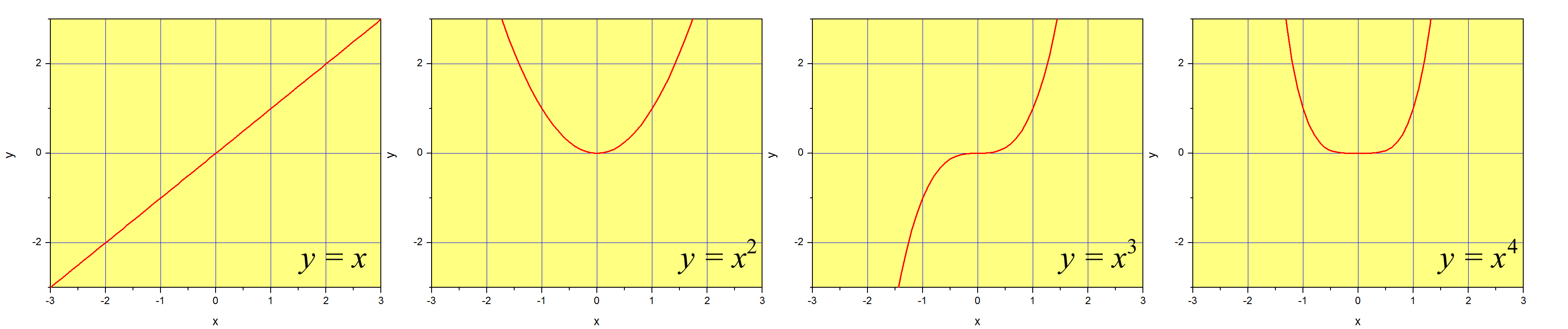
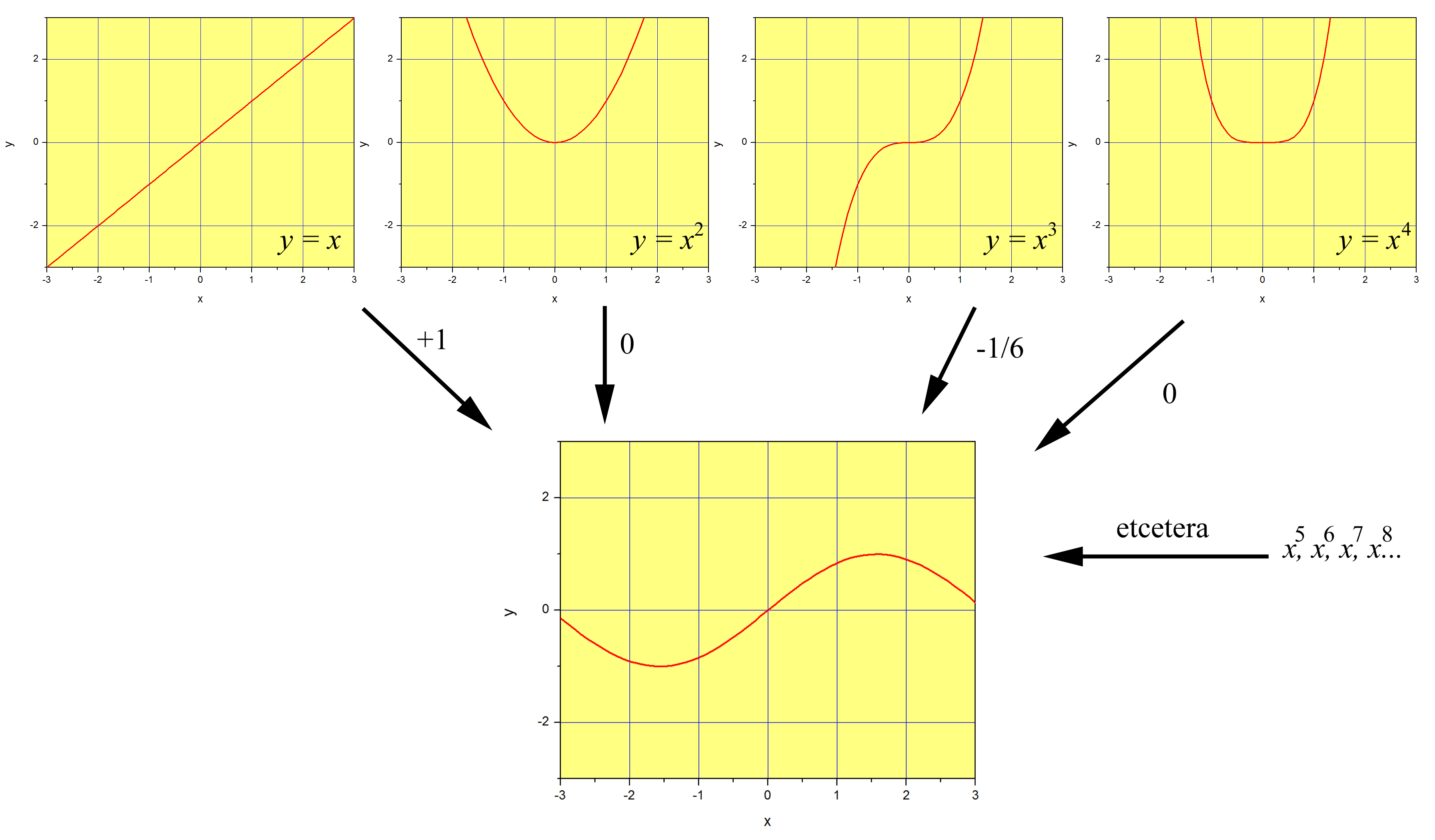
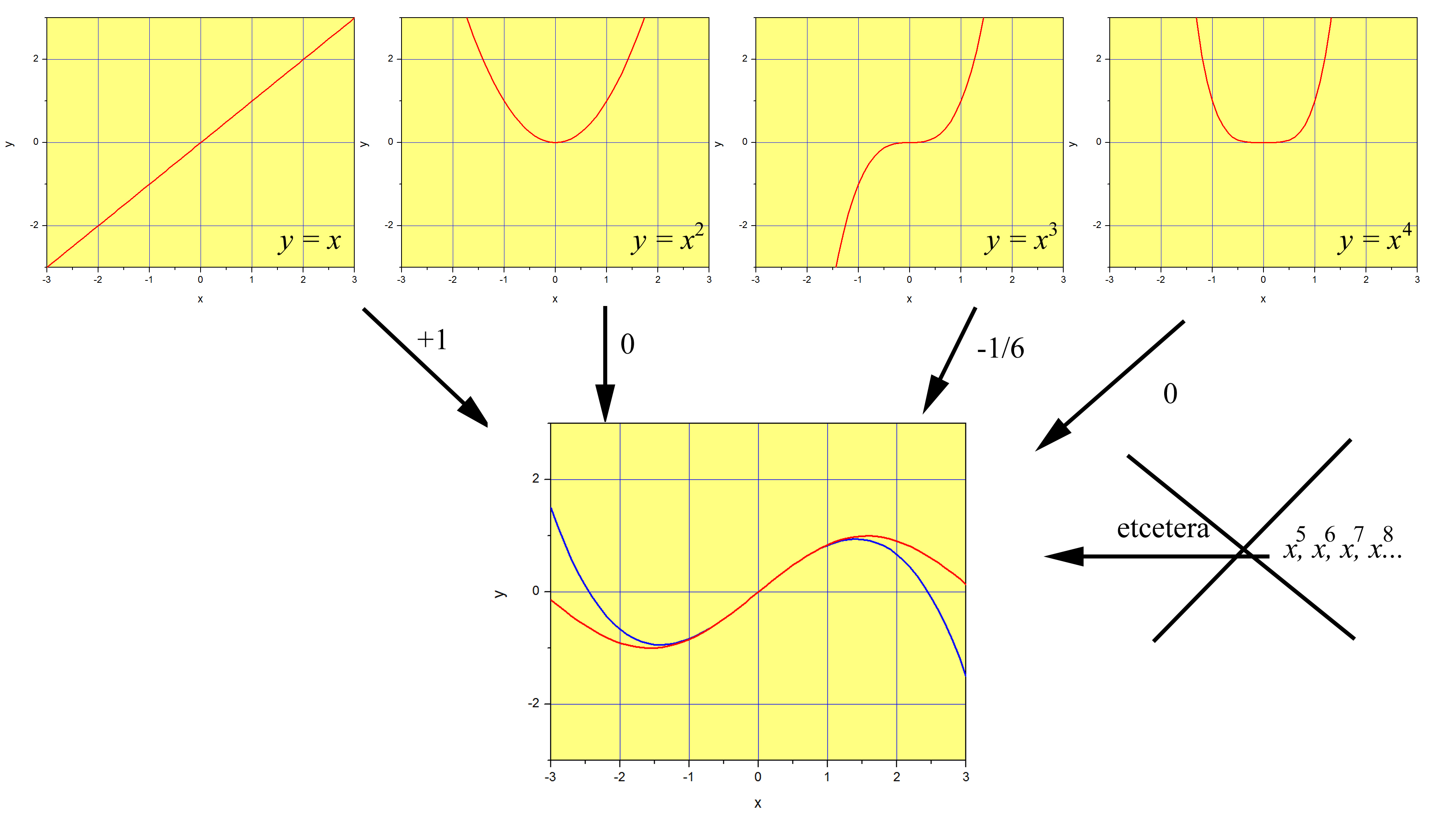
Figure \(\PageIndex{1}\) is a graphic representation of the first four functions of this basis set. To be fair, the first function of the set is \(x^0=1\), so these would be the second, third, fourth and fifth. The full basis set is of course infinite in length. If we mix all the functions of the set with equal weights (we put the same amount of \(x^2\) than we put \(x^{245}\) or \(x^{0}\)), we obtain \((1-x)^{-1}\) (Equation \ref{eq1}. If we use only the odd terms, alternate the sign starting with a ‘+’, and weigh each term less and less using the expression \(1/(2n-1)!\) for the \(n-th\) term, we obtain \(\sin{x}\) (Equation \ref{series:sin}). This is illustrated in Figure \(\PageIndex{2}\), where we multiply the even powers of \(x\) by zero, and use different weights for the rest. Note that the ‘etcetera’ is crucial, as we would need to include an infinite number of functions to obtain the function \(\sin{x}\) exactly.
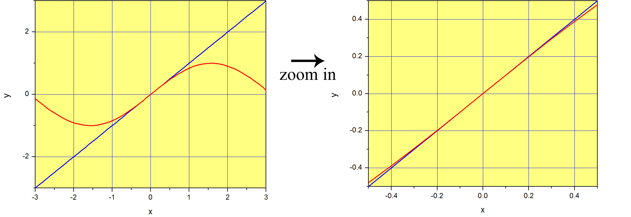
Although we need an infinite number of terms to express a function exactly (unless the function is a polynomial, of course), in many cases we will observe that the weight (the coefficient) of each power of \(x\) gets smaller and smaller as we increase the power. For example, in the case of \(\sin{x}\), the contribution of \(x^3\) is \(1/6 th\) of the contribution of \(x\) (in absolute terms), and the contribution of \(x^5\) is \(1/120 th\). This tells you that the first terms are much more important than the rest, although all are needed if we want the sum to represent \(\sin{x}\) exactly. What if we are happy with a ‘pretty good’ approximation of \(\sin{x}\)? Let’s see what happens if we use up to \(x^3\) and drop the higher terms. The result is plotted in blue in Figure \(\PageIndex{3}\) together with \(\sin{x}\) in red. We can see that the function \(x-1/6 x^3\) is a very good approximation of \(\sin{x}\) as long as we stay close to \(x=0\). As we move further away from the origin the approximation gets worse and worse, and we would need to include higher powers of \(x\) to get it better. This should be clear from eq. [series:sin], since the terms \(x^n\) get smaller and smaller with increasing \(n\) if \(x\) is a small number. Therefore, if \(x\) is small, we could write \(\sin (x) \approx x - \dfrac{1}{3!} x^3\), where the symbol \(\approx\) means approximately equal.
But why stopping at \(n=3\) and not \(n=1\) or 5? The above argument suggests that the function \(x\) might be a good approximation of \(\sin{x}\) around \(x=0\), when the term \(x^3\) is much smaller than the term \(x\). This is in fact this is the case, as shown in Figure \(\PageIndex{4}\).
We have seen that we can get good approximations of a function by truncating the series (i.e. not using the infinite terms). Students usually get frustrated and want to know how many terms are ‘correct’. It takes a little bit of practice to realize there is no universal answer to this question. We would need some context to analyze how good of an approximation we are happy with. For example, are we satisfied with the small error we see at \(x= 0.5\) in Figure \(\PageIndex{4}\)? It all depends on the context. Maybe we are performing experiments where we have other sources of error that are much worse than this, so using an extra term will not improve the overall situation anyway. Maybe we are performing very precise experiments where this difference is significant. As you see, discussing how many terms are needed in an approximation out of context is not very useful. We will discuss this particular approximation when we learn about second order differential equations and analyze the problem of the pendulum, so hopefully things will make more sense then.
Linear Approximations
If you take a look at Equation \(3.1.5\) you will see that we can always approximate a function as \(a_0+a_1x\) as long as \(x\) is small. When we say ‘any function’ we of course imply that the function and all its derivatives need to be finite at \(x=0\). Looking at the definitions of the coefficients, we can write:
\[\label{eq1} f (x) \approx f(0) +f'(0)x \]
We call this a linear approximation because Equation \ref{eq1} is the equation of a straight line. The slope of this line is \(f'(0)\) and the \(y\)-intercept is \(f(0)\).
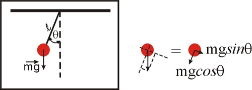
A fair question at this point is ‘why are we even talking about approximations?’ What is so complicated about the functions \(\sin{x}\), \(e^x\) or \(\ln{(x+1)}\) that we need to look for an approximation? Are we getting too lazy? To illustrate this issue, let’s consider the problem of the pendulum, which we will solve in detail in the chapter devoted to differential equations. The problem is illustrated in Figure \(\PageIndex{1}\), and those of you who took a physics course will recognize the equation below, which represents the law of motion of a simple pendulum. The second derivative refers to the acceleration, and the \(\sin \theta\) term is due to the component of the net force along the direction of motion. We will discuss this in more detail later in this semester, so for now just accept the fact that, for this system, Newton’s law can be written as:
\[\frac{d^2\theta(t)}{dt^2}+\frac{g}{l} \sin{\theta(t)}=0 \nonumber \]
This equation should be easy to solve, right? It has only a few terms, nothing too fancy other than an innocent sine function...How difficult can it be to obtain \(\theta(t)\)? Unfortunately, this differential equation does not have an analytical solution! An analytical solution means that the solution can be expressed in terms of a finite number of elementary functions (such as sine, cosine, exponentials, etc). Differential equations are sometimes deceiving in this way: they look simple, but they might be incredibly hard to solve, or even impossible! The fact that we cannot write down an analytical solution does not mean there is no solution to the problem. You can swing a pendulum and measure \(\theta(t)\) and create a table of numbers, and in principle you can be as precise as you want to be. Yet, you will not be able to create a function that reflects your numeric results. We will see that we can solve equations like this numerically, but not analytically. Disappointing, isn’t it? Well... don’t be. A lot of what we know about molecules and chemical reactions came from the work of physical chemists, who know how to solve problems using numerical methods. The fact that we cannot obtain an analytical expression that describes a particular physical or chemical system does not mean we cannot solve the problem numerically and learn a lot anyway!
But what if we are interested in small displacements only (that is, the pendulum swings close to the vertical axis at all times)? In this case, \(\theta<<1\), and as we saw \(\sin{\theta}\approx\theta\) (see Figure \(3.1.4\)). If this is the case, we have now:
\[\frac{d^2\theta(t)}{dt^2}+\frac{g}{l} \theta(t)=0 \nonumber \]
As it turns out, and as we will see in Chapter 2, in this case it is very easy to obtain the solution we are looking for:
\[\theta(t)=\theta(t=0)\cos \left((\frac{g}{l})^{1/2}t \right) \nonumber \]
This solution is the familiar ‘back and forth’ oscillatory motion of the pendulum you are familiar with. What you might have not known until today is that this solution assumes \(\sin{\theta}\approx\theta\) and is therefore valid only if \(\theta<<1\)!
There are lots of ‘hidden’ linear approximations in the equations you have learned in your physics and chemistry courses. You may recall your teachers telling you that a give equation is valid only at low concentrations, or low pressures, or low... you hopefully get the point. A pendulum is of course not particularly interesting when it comes to chemistry, but as we will see through many examples during the semester, oscillations, generally speaking, are. The example below illustrates the use of series to a problem involving diatomic molecules, but before discussing it we need to provide some background.
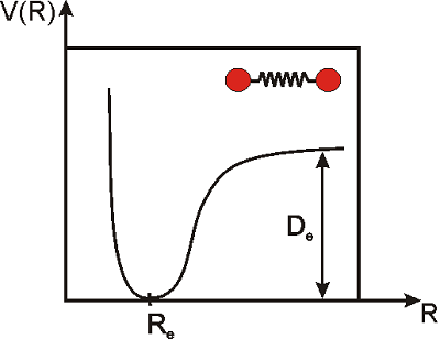
The vibrations of a diatomic molecule are often modeled in terms of the so-called Morse potential. This equation does not provide an exact description of the vibrations of the molecule under any condition, but it does a pretty good job for many purposes.
\[\label{morse}V(R)=D_e\left(1-e^{-k(R-R_e)}\right)^2 \]
Here, \(R\) is the distance between the nuclei of the two atoms, \(R_e\) is the distance at equilibrium (i.e. the equilibrium bond length), \(D_e\) is the dissociation energy of the molecule, \(k\) is a constant that measures the strength of the bond, and \(V\) is the potential energy. Note that \(R_e\) is the distance at which the potential energy is a minimum, and that is why we call this the equilibrium distance. We would need to apply energy to separate the atoms even more, or to push them closer (Figure \(\PageIndex{2}\)).
At room temperature, there is enough thermal energy to induce small vibrations that displace the atoms from their equilibrium positions, but for stable molecules, the displacement is very small: \(R-R_e\rightarrow0\). In the next example we will prove that under these conditions, the potential looks like a parabola, or in mathematical terms, \(V(R)\) is proportional to the square of the displacement. This type of potential is called a ’harmonic potential’. A vibration is said to be simple harmonic if the potential is proportional to the square of the displacement (as in the simple spring problems you may have studied in physics).
Expand the Morse potential as a power series and prove that the vibrations of the molecule are approximately simple harmonic if the displacement \(R-R_e\) is small.
Solution
The relevant variable in this problem is the displacement \(R-R_e\), not the actual distance \(R\). Let’s call the displacement \(R-R_e=x\), and let’s rewrite Equation \ref{morse} as
\[\label{morse2}V(R)=D_e\left(1-e^{-kx}\right)^2 \]
The goal is to prove that \(V(R) =cx^2\) (i.e. the potential is proportional to the square of the displacement) when \(x\rightarrow0\). The constant \(c\) is the proportionality constant. We can approach this in two different ways. One option is to expand the function shown in Equation \ref{morse2} around zero. This would be correct, but it but involve some unnecessary work. The variable \(x\) appears only in the exponential term, so a simpler option is to expand the exponential function, and plug the result of this expansion back in Equation \ref{morse2}. Let’s see how this works:
We want to expand \(e^{-kx}\) as \(a_0+a_1 x + a_2 x^2...a_n x^n\), and we know that the coefficients are \(a_n=\frac{1}{n!} \left( \frac{d^n f(x)}{dx^n} \right)_0.\)
The coefficient \(a_0\) is \(f(0)=1\). The first three derivatives of \(f(x)=e^{-kx}\) are
- \(f'(x)=-ke^{-kx}\)
- \(f''(x)=k^2e^{-kx}\)
- \(f'''(x)=-k^3e^{-kx}\)
When evaluated at \(x=0\) we obtain, \(-k, k^2, -k^3...\)
and therefore \(a_n=\frac{(-1)^n k^n}{n!}\) for \(n=0, 1, 2...\).
Therefore,
\[e^{-kx}=1-kx+k^2x^2/2!-k^3x^3/3!+k^4x^4/4!... \nonumber \]
and
\[1-e^{-kx}=+kx-k^2x^2/2!+k^3x^3/3!-k^4x^4/4!... \nonumber \]
From the last result, when \(x<<1\), we know that the terms in \(x^2, x^3...\) will be increasingly smaller, so \(1-e^{-kx}\approx kx\) and \((1-e^{-kx})^2\approx k^2x^2\).
Plugging this result in Equation \ref{morse2} we obtain \(V(R) \approx D_e k^2 x^2\), so we demonstrated that the potential is proportional to the square of the displacement when the displacement is small (the proportionality constant is \(D_e k^2\)). Therefore, stable diatomic molecules at room temperatures behave pretty much like a spring! (Don’t take this too literally. As we will discuss later, microscopic springs do not behave like macroscopic springs at all).
Taylor Series
Before discussing more applications of Maclaurin series, let’s expand our discussion to the more general case where we expand a function around values different from zero. Let’s say that we want to expand a function around the number \(h\). If \(h=0\), we call the series a Maclaurin series, and if \(h\neq0\) we call the series a Taylor series. Because Maclaurin series are a special case of the more general case, we can call all the series Taylor series and omit the distinction. The following is true for a function \(f(x)\) as long as the function and all its derivatives are finite at \(h\):
\[\label{taylor} f(x)=a_0 + a_1(x-h)+a_2(x-h)^2+...+a_n(x-h)^n = \displaystyle\sum_{n=0}^{\infty}a_n(x-h)^n \]
The coefficients are calculated as
\[\label{taylorcoeff} a_n=\frac{1}{n!}\left( \frac{d^n f}{dx^n}\right)_h \]
Notice that instead of evaluating the function and its derivatives at \(x=0\) we now evaluate them at \(x=h\), and that the basis set is now \(1, (x-h), (x-h)^2,...,(x-h)^n\) instead of \(1, x, x^2,...,x^n\). A Taylor series will be a good approximation of the function at values of \(x\) close to \(h\), in the same way Maclaurin series provide good approximations close to zero.
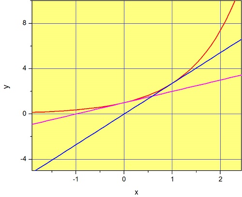
To see how this works let’s go back to the exponential function. Recall that the Maclaurin expansion of \(e^x\) is shown in Equation \(3.1.3\). We know what happens if we expand around zero, so to practice, let’s expand around \(h=1\). The coefficient \(a_0\) is \(f(1)= e^1=e\). All the derivatives are \(e^x\), so \(f'(1)=f''(1)=f'''(1)...=e.\) Therefore, \(a_n=\frac{e}{n!}\) and the series is therefore
\[\label{taylorexp} e\left[ 1+(x-1)+\frac{1}{2}(x-1)^2+\frac{1}{6}(x-1)^3+... \right]=\displaystyle\sum_{n=0}^{\infty}\frac{e}{n!}(x-1)^n \]
We can use the same arguments we used before to conclude that \(e^x\approx ex\) if \(x\approx 1\). If \(x\approx 1\), \((x-1)\approx 0\), and the terms \((x-1)^2, (x-1)^3\) will be smaller and smaller and will contribute less and less to the sum. Therefore,
\[e^x \approx e \left[ 1+(x-1) \right]=ex. \nonumber \]
This is the equation of a straight line with slope \(e\) and \(y\)-intercept 0. In fact, from Equation \(3.1.7\) we can see that all functions will look linear at values close to \(h\). This is illustrated in Figure \(\PageIndex{1}\), which shows the exponential function (red) together with the functions \(1+x\) (magenta) and \(ex\) (blue). Not surprisingly, the function \(1+x\) provides a good approximation of \(e^x\) at values close to zero (see Equation \(3.1.3\)) and the function \(ex\) provides a good approximation around \(x=1\) (Equation \ref{taylorexp}).
Expand \(f(x)=\ln{x}\) about \(x=1\)
Solution
\[f(x)=a_0 + a_1(x-h)+a_2(x-h)^2+...+a_n(x-h)^n, a_n=\frac{1}{n!}\left( \frac{d^n f}{dx^n}\right)_h \nonumber \]
\[a_0=f(1)=\ln(1)=0 \nonumber \]
The derivatives of \(\ln{x}\) are:
\[f'(x) = 1/x, f''(x)=-1/x^2, f'''(x) = 2/x^3, f^{(4)}(x)=-6/x^4, f^{(5)}(x)=24/x^5... \nonumber \]
and therefore,
\[f'(1) = 1, f''(1)=-1, f'''(1) = 2, f^{(4)}(1)=-6, f^{(5)}(1)=24.... \nonumber \]
To calculate the coefficients, we need to divide by \(n!\):
- \(a_1=f'(1)/1!=1\)
- \(a_2=f''(1)/2!=-1/2\)
- \(a_3=f'''(1)/3!=2/3!=1/3\)
- \(a_4=f^{(4)}(1)/4!=-6/4!=-1/4\)
- \(a_n=(-1)^{n+1}/n\)
The series is therefore:
\[f(x)=0 + 1(x-1)-1/2 (x-1)^2+1/3 (x-1)^3...=\displaystyle{\color{Maroon}\displaystyle\sum_{n=1}^{\infty} \frac{(-1)^{n+1}}{n}(x-1)^{n}} \nonumber \]
Note that we start the sum at \(n=1\) because \(a_0=0\), so the term for \(n=0\) does not have any contribution.
Need help? The links below contain solved examples.
External links:
Finding the Taylor series of a function I: http://patrickjmt.com/taylor-and-maclaurin-series-example-2/