
30.10: The Potential-Energy Surface Can Be Calculated Using Quantum Mechanics
- Page ID
- 14571
\( \newcommand{\vecs}[1]{\overset { \scriptstyle \rightharpoonup} {\mathbf{#1}} } \)
\( \newcommand{\vecd}[1]{\overset{-\!-\!\rightharpoonup}{\vphantom{a}\smash {#1}}} \)
\( \newcommand{\id}{\mathrm{id}}\) \( \newcommand{\Span}{\mathrm{span}}\)
( \newcommand{\kernel}{\mathrm{null}\,}\) \( \newcommand{\range}{\mathrm{range}\,}\)
\( \newcommand{\RealPart}{\mathrm{Re}}\) \( \newcommand{\ImaginaryPart}{\mathrm{Im}}\)
\( \newcommand{\Argument}{\mathrm{Arg}}\) \( \newcommand{\norm}[1]{\| #1 \|}\)
\( \newcommand{\inner}[2]{\langle #1, #2 \rangle}\)
\( \newcommand{\Span}{\mathrm{span}}\)
\( \newcommand{\id}{\mathrm{id}}\)
\( \newcommand{\Span}{\mathrm{span}}\)
\( \newcommand{\kernel}{\mathrm{null}\,}\)
\( \newcommand{\range}{\mathrm{range}\,}\)
\( \newcommand{\RealPart}{\mathrm{Re}}\)
\( \newcommand{\ImaginaryPart}{\mathrm{Im}}\)
\( \newcommand{\Argument}{\mathrm{Arg}}\)
\( \newcommand{\norm}[1]{\| #1 \|}\)
\( \newcommand{\inner}[2]{\langle #1, #2 \rangle}\)
\( \newcommand{\Span}{\mathrm{span}}\) \( \newcommand{\AA}{\unicode[.8,0]{x212B}}\)
\( \newcommand{\vectorA}[1]{\vec{#1}} % arrow\)
\( \newcommand{\vectorAt}[1]{\vec{\text{#1}}} % arrow\)
\( \newcommand{\vectorB}[1]{\overset { \scriptstyle \rightharpoonup} {\mathbf{#1}} } \)
\( \newcommand{\vectorC}[1]{\textbf{#1}} \)
\( \newcommand{\vectorD}[1]{\overrightarrow{#1}} \)
\( \newcommand{\vectorDt}[1]{\overrightarrow{\text{#1}}} \)
\( \newcommand{\vectE}[1]{\overset{-\!-\!\rightharpoonup}{\vphantom{a}\smash{\mathbf {#1}}}} \)
\( \newcommand{\vecs}[1]{\overset { \scriptstyle \rightharpoonup} {\mathbf{#1}} } \)
\( \newcommand{\vecd}[1]{\overset{-\!-\!\rightharpoonup}{\vphantom{a}\smash {#1}}} \)
\(\newcommand{\avec}{\mathbf a}\) \(\newcommand{\bvec}{\mathbf b}\) \(\newcommand{\cvec}{\mathbf c}\) \(\newcommand{\dvec}{\mathbf d}\) \(\newcommand{\dtil}{\widetilde{\mathbf d}}\) \(\newcommand{\evec}{\mathbf e}\) \(\newcommand{\fvec}{\mathbf f}\) \(\newcommand{\nvec}{\mathbf n}\) \(\newcommand{\pvec}{\mathbf p}\) \(\newcommand{\qvec}{\mathbf q}\) \(\newcommand{\svec}{\mathbf s}\) \(\newcommand{\tvec}{\mathbf t}\) \(\newcommand{\uvec}{\mathbf u}\) \(\newcommand{\vvec}{\mathbf v}\) \(\newcommand{\wvec}{\mathbf w}\) \(\newcommand{\xvec}{\mathbf x}\) \(\newcommand{\yvec}{\mathbf y}\) \(\newcommand{\zvec}{\mathbf z}\) \(\newcommand{\rvec}{\mathbf r}\) \(\newcommand{\mvec}{\mathbf m}\) \(\newcommand{\zerovec}{\mathbf 0}\) \(\newcommand{\onevec}{\mathbf 1}\) \(\newcommand{\real}{\mathbb R}\) \(\newcommand{\twovec}[2]{\left[\begin{array}{r}#1 \\ #2 \end{array}\right]}\) \(\newcommand{\ctwovec}[2]{\left[\begin{array}{c}#1 \\ #2 \end{array}\right]}\) \(\newcommand{\threevec}[3]{\left[\begin{array}{r}#1 \\ #2 \\ #3 \end{array}\right]}\) \(\newcommand{\cthreevec}[3]{\left[\begin{array}{c}#1 \\ #2 \\ #3 \end{array}\right]}\) \(\newcommand{\fourvec}[4]{\left[\begin{array}{r}#1 \\ #2 \\ #3 \\ #4 \end{array}\right]}\) \(\newcommand{\cfourvec}[4]{\left[\begin{array}{c}#1 \\ #2 \\ #3 \\ #4 \end{array}\right]}\) \(\newcommand{\fivevec}[5]{\left[\begin{array}{r}#1 \\ #2 \\ #3 \\ #4 \\ #5 \\ \end{array}\right]}\) \(\newcommand{\cfivevec}[5]{\left[\begin{array}{c}#1 \\ #2 \\ #3 \\ #4 \\ #5 \\ \end{array}\right]}\) \(\newcommand{\mattwo}[4]{\left[\begin{array}{rr}#1 \amp #2 \\ #3 \amp #4 \\ \end{array}\right]}\) \(\newcommand{\laspan}[1]{\text{Span}\{#1\}}\) \(\newcommand{\bcal}{\cal B}\) \(\newcommand{\ccal}{\cal C}\) \(\newcommand{\scal}{\cal S}\) \(\newcommand{\wcal}{\cal W}\) \(\newcommand{\ecal}{\cal E}\) \(\newcommand{\coords}[2]{\left\{#1\right\}_{#2}}\) \(\newcommand{\gray}[1]{\color{gray}{#1}}\) \(\newcommand{\lgray}[1]{\color{lightgray}{#1}}\) \(\newcommand{\rank}{\operatorname{rank}}\) \(\newcommand{\row}{\text{Row}}\) \(\newcommand{\col}{\text{Col}}\) \(\renewcommand{\row}{\text{Row}}\) \(\newcommand{\nul}{\text{Nul}}\) \(\newcommand{\var}{\text{Var}}\) \(\newcommand{\corr}{\text{corr}}\) \(\newcommand{\len}[1]{\left|#1\right|}\) \(\newcommand{\bbar}{\overline{\bvec}}\) \(\newcommand{\bhat}{\widehat{\bvec}}\) \(\newcommand{\bperp}{\bvec^\perp}\) \(\newcommand{\xhat}{\widehat{\xvec}}\) \(\newcommand{\vhat}{\widehat{\vvec}}\) \(\newcommand{\uhat}{\widehat{\uvec}}\) \(\newcommand{\what}{\widehat{\wvec}}\) \(\newcommand{\Sighat}{\widehat{\Sigma}}\) \(\newcommand{\lt}{<}\) \(\newcommand{\gt}{>}\) \(\newcommand{\amp}{&}\) \(\definecolor{fillinmathshade}{gray}{0.9}\)A potential energy surface (PES) describes the potential energy of a system, especially a collection of atoms, in terms of certain parameters, normally the positions of the atoms. The surface might define the energy as a function of one or more coordinates; if there is only one coordinate, the surface is called a potential energy curve or energy profile. It is helpful to use the analogy of a landscape: for a system with two degrees of freedom (e.g. two bond lengths), the value of the energy (analogy: the height of the land) is a function of two bond lengths (analogy: the coordinates of the position on the ground). The Potential Energy Surface represents the concept that each geometry (both external and internal) of the atoms of the molecules in a chemical reaction has associated with it a unique potential energy. This creates a smooth energy “landscape” and chemistry can be viewed from a topology perspective of particles evolving as they pass through potential energy "valleys" and "passes".
The PES concept finds application in fields such as chemistry and physics, especially in the theoretical sub-branches of these subjects. It can be used to theoretically explore properties of structures composed of atoms, for example, finding the minimum energy shape of a molecule or computing the rates of a chemical reaction.
Potential Energy Curves (2-D Potential Energy Surfaces)
The energy of a system of two atoms depends on the distance between them. At large distances the energy is zero, meaning “no interaction”. At distances of several atomic diameters, attractive forces dominate, whereas at very close approaches the force is repulsive, causing the energy to rise. The attractive and repulsive effects are balanced at the minimum point in the curve. Plots that illustrate this relationship are quite useful in defining certain properties of a chemical bond (Figure \(\PageIndex{1}\)).

The internuclear distance at which the potential energy minimum occurs defines the bond length. This is more correctly known as the equilibrium bond length because thermal motion causes the two atoms to vibrate about this distance. In general, the stronger the bond, the smaller the bond length.
Attractive forces operate between all atoms, but unless the potential energy minimum is at least of the order of RT, the two atoms will not be able to withstand the disruptive influence of thermal energy long enough to result in an identifiable molecule. Thus we can say that a chemical bond exists between the two atoms in H2. The weak attraction between argon atoms does not allow Ar2 to exist as a molecule, but it does give rise to the van der Waals force that holds argon atoms together in their liquid and solid forms.
Potential energy and kinetic energy quantum theory tell us that an electron in an atom possesses kinetic energy \(K\) as well as potential energy \(V\), so the total energy \(E\) is always the sum of the two: \(E = V + K\). The relation between them is surprisingly simple: \(K = –0.5 V\). This means that when a chemical bond forms (an exothermic process with \(ΔE < 0\)), the decrease in potential energy is accompanied by an increase in the kinetic energy (embodied in the momentum of the bonding electrons), but the magnitude of the latter change is only half as much, so the change in potential energy always dominates. The bond energy \(–ΔE\) has half the magnitude of the decrease in potential energy.
Mathematical Definition and Computation of a Potential Energy Surface
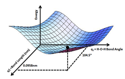
The geometry of a set of atoms can be described by a vector, r, whose elements represent the atom positions. The vector \(r\) could be the set of the Cartesian coordinates of the atoms, or could also be a set of inter-atomic distances and angles. Given \(r\), the energy as a function of the positions, \(V(r)\), is the value of \(V(r)\) for all values of \(r\) of interest. Using the landscape analogy from the introduction, \(V(r)\) gives the height on the "energy landscape" so that the concept of a potential energy surface arises. An example is the PES for water molecule (Figure \(\PageIndex{2}\)) that shows the energy minimum corresponding to optimized molecular structure for water- O-H bond lengths of 0.0958 nm and H-O-H bond angle of 104.5°
To define an atom’s location in 3-dimensional space requires three coordinates (e.g., \(x\), \(y\),and \(z\) or \(r\), \(\theta\) and \(phi\) in Cartesian and Spherical coordinates) or degrees of freedom. However, a reaction and hence the corresponding PESs do not depend on the absolute position of the reaction, only the relative positions (internal degrees). Hence both translation and rotation of the entire system can be removed (each with 3 degrees of freedom, assuming non-linear geometries). So the dimensionality of a PES is
\[3N-6\nonumber \]
where \(N\) is the number of atoms involves in the reaction, i.e., the number of atoms in each reactant). The PES is a hypersurface with many degrees of freedom and typically only a few are plotted at any one time for understanding. See Calculate Number of Vibrational Modes to get a more detailed picture of how this applies to calculating the number of vibrations in a molecule
To study a chemical reaction using the PES as a function of atomic positions, it is necessary to calculate the energy for every atomic arrangement of interest. Methods of calculating the energy of a particular atomic arrangement of atoms are well known. For very simple chemical systems or when simplifying approximations are made about inter-atomic interactions, it is sometimes possible to use an analytically derived expression for the energy as a function of the atomic positions. An example is
\[\ce{H + H_2 -> H_2 + H}\label{30.10.1} \]
a system that is described by a function of the three \(\ce{H-H}\) distances. For more complicated systems, calculation of the energy of a particular arrangement of atoms is often too computationally expensive for large-scale representations of the surface to be feasible.
Applications of Potential Energy Surfaces
A PES is a conceptual tool for aiding the analysis of molecular geometry and chemical reaction dynamics. Once the necessary points are evaluated on a PES, the points can be classified according to the first and second derivatives of the energy with respect to position, which respectively are the gradient and the curvature. Stationary points (or points with a zero gradient) have physical meaning: energy minima correspond to physically stable chemical species and saddle points correspond to transition states, the highest energy point on the reaction coordinate (which is the lowest energy pathway connecting a chemical reactant to a chemical product).
A Hypothetical Endothermic Reaction PES
Figure \(\PageIndex{3}\) shows an example of a PES for a hypothetical reaction system, with the corresponding 2-D energy contour map projected on the plane below. The contour map shows isolines of potential energy, using color to differentiate between high and low energies. In this figure, the highest potential energy is indicated with red, and as the color changes along the ROYGBIV scale, the potential energy decreases until violet is reached, indicating the lowest potential energy. In the PES, the \(z\) axis represents the potential energy, with the energy of the plane in the PES defined as 0 kJ. The color scheme of the PES has the same meaning as that of the 2-D contour map - red is high potential energy and violet is low potential energy.

Before the reaction, the reactants are found at (or near) the energy minimum on the right. (The deep well in the PES and the smallest, violet oval in the contour map.) As the reaction proceeds, the reactants are shown following the minimum energy pathway toward the products, as designated by the dashed red line. The point "2" designates the transition state at the saddle point, the highest energy point of the reaction process. The reaction then moves on to form the products, which sit in the potential energy well on the left. (Designated by the shallower well on the PES and by the dark blue oval on the left in the contour map.) Because the potential energy of the reactants is greater than the potential energy of the products, this reaction is an endothermic reaction. The point "1" represents a second, higher energy saddle point which is the transition state for an alternative reaction that is possible for this set of chemicals.
The Exchange Reaction HA + HBHC ⇒ HAHB + HC
A specific application of a PES is the mapping of the reaction shown in equation \(\ref{30.10.1}\), the exchange of hydrogen atoms in an H2 molecule. In this map, the individual H atoms are labeled as
\[H_A + H_BH_C \rightarrow H_AH_B + H_C \nonumber \]
We must take into account the collision angle between the \(H_A\) atom and the \(H_BH_C\) molecule. If we fix this collision angle at 180°, we are able to plot a PES that is dependent on the two parameters of \(R_{BC}\) and \(R_{AB}\). The resulting PES (figure \(\PageIndex{4a}\)) and energy contour map (figure \(\PageIndex{4b}\)) show us that if the particles are far enough apart, the potential energy of the reaction system starts out being described by the potential energy curve for the \(H_BH_C\) molecule, and ends up being described by the potential energy curve of the \(H_AH_B \) molecule. Individually, these curves both have appearances similar to the curve shown in Figure \(\PageIndex{1}\). The PES and the energy contour map show the symmetrical nature of the potential energy changes that occur in this exchange process that involves products that are equivalent to the reactants.


As the \(H_A\) atom more closely approaches the \(H_BH_C\) molecule, the interactions between these particles begin to affect the potential energy of the system. There are many possible potential energy pathways that the reaction could follow. Figure \(\PageIndex{5}\) shows the energy contour map for three possible reaction pathways:

In pathway 1, the \(H_BH_C\) bond length \(R_{BC} \) is held constant as the distance \(R_{AB}\) decreases. This type of interaction would lead to a continually increasing potential energy for the system as the \(H_A\) atom moves closer and closer to the \(H_BH_C\) molecule. Eventually, the new \(H_AH_B\) molecule would form, and the \(H_C\) atom would break off and would move farther and farther away.
Pathway 2 shows a second possible reaction pathway in which the \(H_BH_C\) bond length \(R_{BC} \) increases even though the \(H_A\) atom is still relatively far away. This pathway is unlikely because it requires a great deal of potential energy to stretch the \(H_BH_C\) bond before the attractive force from the \(H_A\) atom influences this bond lengthening.
As the particles travel along Pathway 3, the reactants still must pass through a potential energy maximum at the saddle point, but this local maximum is the lowest energy barrier separating reactants from products. As noted above, this saddle point is called the transition state structure (designated by the red dot in pathway 3). This is the structure that is equally poised to return to the reactants or move forward to form products. Pathway 3 is the minimum energy pathway, and thus the one most likely to be followed during a successful reaction.
It is sometimes useful to create energy contour maps that include information about the vibrational state of reactants and products, as shown in figure \(\PageIndex{6}\).

The Exchange Reaction F + D2 ⇒ DF + D
When modeling the potential energy for the reaction
\[\ce{F(g) + D_2(g) -> DF(g) + D(g)}\nonumber \]
it is useful to differentiate between the two deuterium atoms, so we can designate them as \(\ce{D}_A\) and \(\ce{D}_B\). Doing so allows us to determine how the potential energy of the pre-reaction system is affected by the \(\ce{F}\) to \(\ce{D}_A\) distance \(R_{\ce{D}_A \ce{F}}\) and the \(\ce{D}_A\) to \(\ce{D}_B\) distance \(R_{\ce{D}_A \ce{D}_B} \) (figure \(\PageIndex{7}\)).

As the \(\ce{F}\) atom more closely approaches the \(\ce{D_2}\) molecule, the interactions between these particles begin to affect the potential energy of the system. There are many possible potential energy pathways that the reaction could follow. Figure \(\PageIndex{8}\) shows the energy contour map for three possible reaction pathways:

In pathway 1, the \(\ce{D_2}\) bond length \(R_{\ce{D}_A \ce{D}_B} \) is held constant as the distance \(R_{\ce{D}_A \ce{F}}\) decreases. This type of interaction would lead to a continually increasing potential energy for the system as the \(\ce{F}\) atom moves closer and closer to the \(\ce{D_2}\) molecule. Eventually, the new \(\ce{D}_A \ce{F}\) molecule would form, and the \(\ce{D}_B\) atom would break off and would move farther and farther away.
Pathway 2 shows a second possible reaction pathway in which the \(\ce{D_2}\) bond length \(R_{\ce{D}_A \ce{D}_B} \) increases even though the F atom is still relatively far away. This pathway is unlikely because it requires a great deal of potential energy to stretch the \(\ce{D_2}\) bond before the attractive force from the F atom influences this bond lengthening.
As the particles travel along Pathway 3, the reactants still must pass through a potential energy maximum at the saddle point, but this local maximum is the lowest energy barrier separating reactants from products. As noted above, this saddle point is called the transition state structure (designated by the red dot in pathway 3, labeled as \(3^{\ddagger}\)). This is the structure that is equally poised to return to the reactants or move forward to form products. Pathway 3 is the minimum energy pathway, and thus the one most likely to be followed during a successful reaction.
If we were to plot the potential energy curve for the reaction pathway along the minimum energy pathway, we would get the familiar potential energy curve of a reaction similar to that shown in Figure \(\PageIndex{9}\).

Contributors and Attributions
- Wikipedia
Stephen Lower, Professor Emeritus (Simon Fraser U.) Chem1 Virtual Textbook
- Tom Neils, Grand Rapids Community College