13.5: Vibrational Overtones

Although the harmonic oscillator proves useful for modeling lower energy levels, like \(v=0, 1\), it fails at higher numbers of \(v\). It not only fails to properly model atomic bonds and dissociations, but also is unable to match spectra showing additional lines that are not accounted for in the harmonic oscillator model.

Anharmonicity

Until this point, we have been using the harmonic oscillator to describe the internuclear potential energy of the vibrational motion. Fundamental vibrational frequencies of a molecule corresponds to a transition of \(\Delta v= \pm 1\). While this is a decent approximation, bonds do not behave like they do in the Harmonic Oscillator approximation (Figure \(\PageIndex{1}\) ). For example, the parabolic potential of the Harmonic Oscillator approximation means that the vibrations can hold any amount of energy and bonds can stretch to any length, while in real molecules if the atoms are too far apart the bond will dissociate.

Figure \(\PageIndex{1}\) : Pictured above is the Harmonic Oscillator approximation (green parabola) superimposed on the anharmonic oscillator (blue curve) on a potential energy diagram. V(R) is the potential energy of a diatomic molecule and R is the radius between the centers of the two atoms. Towards the left is compression of the bond, towards the right is extension. (CC BY-SA 3.0; Created by Mark Somoza March 26 2006).

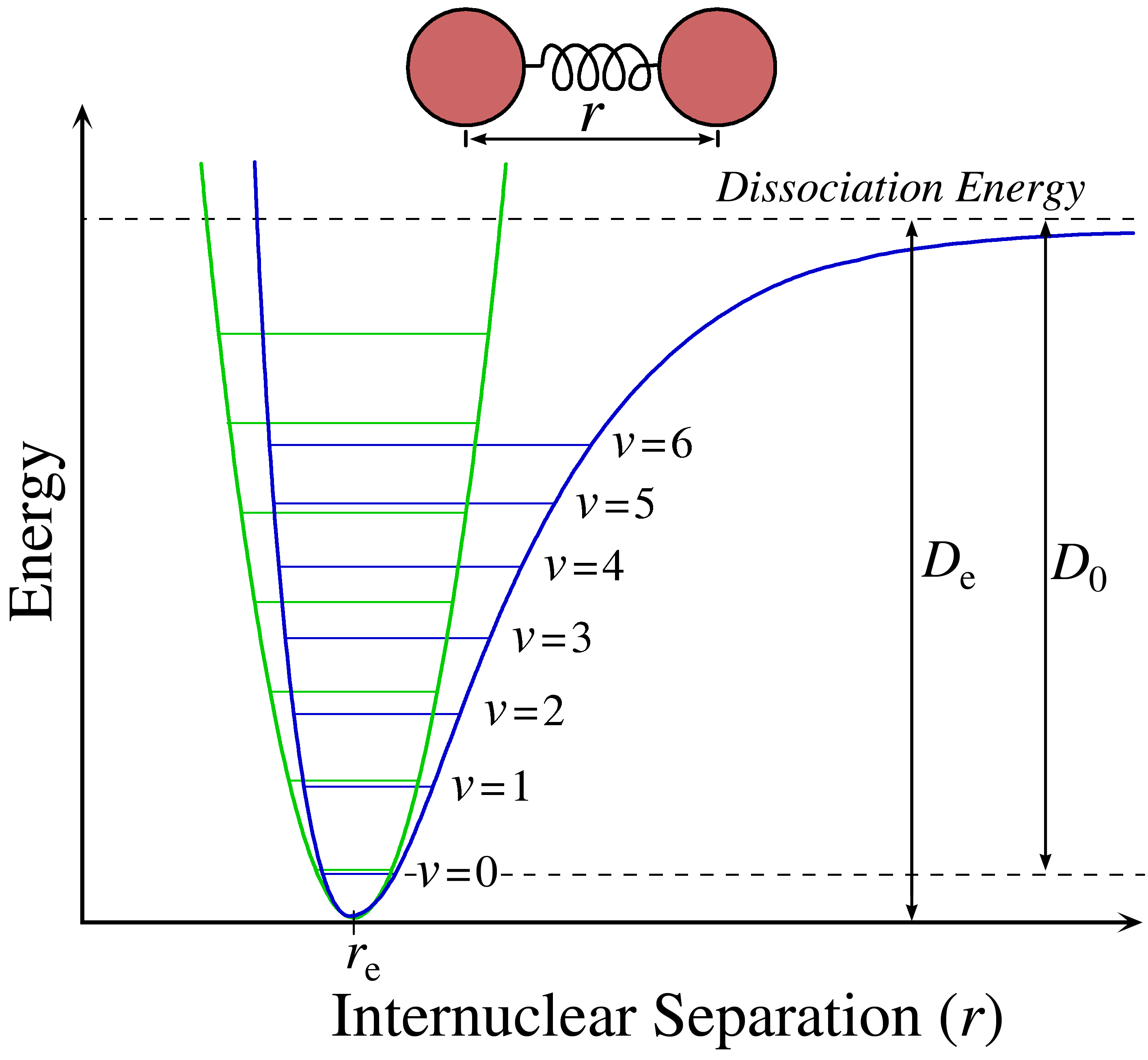
As you can see in Figure \(\PageIndex{1}\) , the harmonic oscillator potential well (in green) only roughly fits over the more accurate anharmonic oscillator well (in blue). The blue curve accounts for dissociation at large R values, which the green curve does not even remotely cover. However, this is just one important difference between the harmonic and anharmonic (real) oscillators.

The real potential energy can be expanded in the Taylor series.

\[ V(R) = V(R_e) + \dfrac{1}{2!}\left(\dfrac{d^2V}{dR^2}\right)_{R=R_e} (R-R_e)^2 + \dfrac{1}{3!}\left(\dfrac{d^3V}{dR^3}\right)_{R=R_e} (R-R_e)^3 + \dfrac{1}{4!}\left(\dfrac{d^4V}{dR^4}\right)_{R=R_e} (R-R_e)^4 + ... \label{taylor} \]

This expansion was discussed in detail previously. The first term in the expansion is ignored since the derivative of the potential at \(R_e\) is zero (i.e., at the bottom of the well). The Harmonic Oscillator approximation only uses the next term, the quadratic term, in the series

\[V_{HO}(R) \approx V(R_e) + \dfrac{1}{2!}\left(\dfrac{d^2V}{dR^2}\right)_{R=R_e} (R-R_e)^2 \nonumber \]

or in terms of a spring constant, ignoring the absolute energy term(\(V(R_e)\)) and defining \(r\) to equal the displacement from equilibrium (\(r=R-R_e\)), then we get the "standard" harmonic oscillator potential:

\[V_{HO}(R) = \dfrac {1}{2} kr^2 \nonumber \]

Alternatively, the expansion in Equation \(\ref{taylor}\) can be shortened to the cubic term

\[V(x) = \dfrac {1}{2} kr^2 + \dfrac {1}{6} \gamma r^3 \label{cubic} \]

where

• \(V(x_0) = 0\), and \(r = R - R_0\).
• \(k\) is the harmonic force constant, and
• \(\gamma\) is the first (i.e., cubic) anharmonic term

It is important to note that this approximation is only good for \(R\) near \(R_0\).

Figure \(\PageIndex{2}\) : (left) Deviation from simple harmonic potential approximation (red curve) of true/exact potential (blue curve) with cubic term (green). (right) Expansion with positive or negative quartic terms. (CC BY-NC; Ümit Kaya via LibreTexts)

The harmonic oscillator approximation gives by the following energies:

\[ E_{v} = \tilde{\nu} \left (v + \dfrac{1}{2} \right) \nonumber \]

When the cubic term in the expansion (Equation \(\ref{cubic}\)) is included, and the Schrödinger equation is solved using perturbation theory this gives:

\[  E_{v} = \tilde{\nu} \left (v + \dfrac{1}{2} \right) - \tilde{\chi_e} \tilde{\nu} \left (v + \dfrac{1}{2} \right)^2 \nonumber \]

where \( \tilde{\chi_e}\) is the anharmonicity constant. It is much smaller than 1, which makes sense because the terms in the Taylor series approach zero. This is why, although \(E_{v}\) technically includes all of the Taylor series, we only concern ourselves with the first and second terms. The rest are so small and barely add to the total and thus can be ignored. To get a more accurate approximation, more terms can be included, but otherwise, can be ignored. Almost all diatomics have experimentally determined \(\frac {d^2 V}{d x^2}\) for their lowest energy states. \(\ce{H2}\), \(\ce{Li2}\), \(\ce{O2}\), \(\ce{N2}\), and \(\ce{F2}\) have had terms up to \(n < 10\) determined of Equation \(\ref{taylor}\).

Overtones

The Harmonic Oscillator approximation predicts that there will be only one line in the spectrum of a diatomic molecule, while experimental data shows there is in fact one dominant line--the fundamental--and other weaker lines. How can we account for these extra lines?

Figure \(\PageIndex{3}\) : A diagram for a vibrating diatomic molecule. The levels denoted by vibrational quantum numbers v represent the potential energy for the harmonic (quadratic) oscillator. The transition \( 0 \rightarrow 1 \) is the fundamental, transitions \( 0 \rightarrow n \) (n>1) are called overtones, and transitions \( 1 \rightarrow n\) (n > 1) are called hot transitions (hot bands).

Any resonant frequency above the fundamental frequency is referred to as an overtone. In the IR spectrum, overtone bands are multiples of the fundamental absorption frequency. As you can recall, the energy levels in the Harmonic Oscillator approximation are evenly spaced apart. Energy is proportional to the frequency absorbed, which in turn is proportional to the wavenumber, the first overtone that appears in the spectrum will be twice the wavenumber of the fundamental. That is, first overtone \(v = 0 \rightarrow 2\) is (approximately) twice the energy of the fundamental, \(v = 0 \rightarrow 1\).

Figure \(\PageIndex{4}\) : An exaggerated view of the energy levels. (a) would be the harmonic oscillator, with the evenly spaced out energy levels. (b) would be the anharmonic, with the energy levels compressing until they converge.

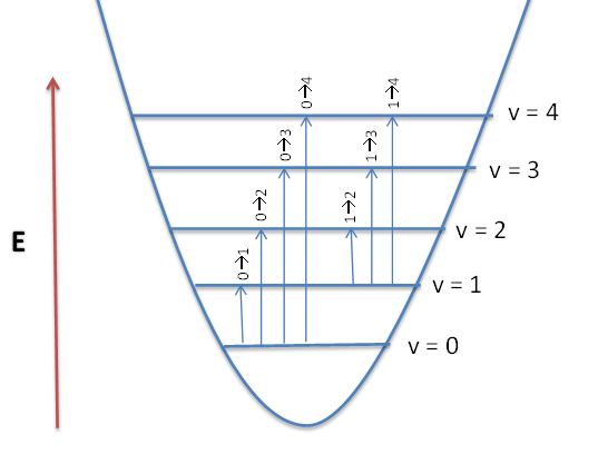
The levels are not equally spaced, like in the harmonic oscillator, but decrease as \(v\) increases, until it ultimately converges, as implied by Figure \(\PageIndex{4}\). Also as a result of anharmonicity, the \(\Delta v= \pm 1\) selection rule is no longer valid and \(v\) can be any number. This leads to the observation of higher order transitions, or overtones, which result from the transition of the ground state to higher energy levels.

Anharmonic Oscillator Selection Rules

For the anharmonic oscillator, the selection rule is \(\Delta V= \text{any number}\). That is, there are no selection rules (for state to state transitions)

Overtones occur when a vibrational mode is excited from \(v=0\) to \(v=2\) (the first overtone) or \(v=0\) to \(v=3\) (the second overtone). The fundamental transitions, \(v=\pm 1\), are the most commonly occurring, and the probability of overtones rapidly decreases as \( \Delta v > \pm 1\) gets bigger. Based on the harmonic oscillator approximation, the energy of the overtone transition will be approximately \(v\) times the fundamental associated with that particular transition. The anharmonic oscillator calculations show that the overtones are usually less than a multiple of the fundamental frequency. Overtones are generally not detected in larger molecules.

This is demonstrated with the vibrations of the diatomic \(\ce{HCl}\) in the gas phase:

Table \(\PageIndex{1}\) : HCl vibrational spectrum.

Transition	ṽobs [cm^-1]	ṽobs Harmonic [cm^-1]	ṽobs Anharmonic [cm^-1]
\( 0 \rightarrow 1 \) (fundamental)	2885.9	2885.9	2,885.3
\( 0 \rightarrow 2 \) (first overtone)	5668.0	5771.8	5,665.0
\( 0 \rightarrow 3 \) (second overtone)	8347.0	8657.7	8,339.0
\( 0 \rightarrow 4\) (third overtone)	10 923.1	11 543.6	10,907.4
\( 0 \rightarrow 5\) (fourth overtone)	13 396.5	14 429.5	13,370

We can see from Table \(\PageIndex{1}\) that the anharmonic frequencies correspond much better with the observed frequencies, especially as the vibrational levels increase. Because the energy levels and overtones are closer together in the anharmonic model, they are also more easily reached. This means that there is a higher chance of that level possibly being occupied, meaning it can show up as additional, albeit weaker intensity lines (the weaker intensity indicates a smaller probability of the transition occuring).

Exercise 13.5.1

\(\ce{HCl}\) has a fundamental band at 2885.9 cm⁻¹ and an overtone at 5668.1 cm⁻¹ Calculate \(\tilde{\nu}\) and \( \tilde{\chi_e} \).

Exercise 13.5.2

Write out the Taylor series, and comment on the trend in the increasing terms. Using a test number \(x\), please add terms 3, 4, and 5, then compare this to term 2. How do they compare? We have seen that the anharmonic terms increase the accuracy of our oscillator approximation. Why don't we care so much about terms past the second?

References

1. Infrared and Raman Spectra of Inorganic and Coordination Compounds. Part A: Theory and Applications in Inorganic Chemistry; Part B: Application in Coordination, Organometallic, and Bioinorganic Chemistry, 5th Edition (Nakamoto, Kazuo)
2. Lyle McAfee Journal of Chemical Education 2000 77 (9), 1122
3. Stuart, Barbara. Infrared Spectroscopy: Fundamentals and Applications. Wiley, 2004. Print.