9.5: Bonding and Antibonding Orbitals
- Page ID
- 13456
\( \newcommand{\vecs}[1]{\overset { \scriptstyle \rightharpoonup} {\mathbf{#1}} } \)
\( \newcommand{\vecd}[1]{\overset{-\!-\!\rightharpoonup}{\vphantom{a}\smash {#1}}} \)
\( \newcommand{\id}{\mathrm{id}}\) \( \newcommand{\Span}{\mathrm{span}}\)
( \newcommand{\kernel}{\mathrm{null}\,}\) \( \newcommand{\range}{\mathrm{range}\,}\)
\( \newcommand{\RealPart}{\mathrm{Re}}\) \( \newcommand{\ImaginaryPart}{\mathrm{Im}}\)
\( \newcommand{\Argument}{\mathrm{Arg}}\) \( \newcommand{\norm}[1]{\| #1 \|}\)
\( \newcommand{\inner}[2]{\langle #1, #2 \rangle}\)
\( \newcommand{\Span}{\mathrm{span}}\)
\( \newcommand{\id}{\mathrm{id}}\)
\( \newcommand{\Span}{\mathrm{span}}\)
\( \newcommand{\kernel}{\mathrm{null}\,}\)
\( \newcommand{\range}{\mathrm{range}\,}\)
\( \newcommand{\RealPart}{\mathrm{Re}}\)
\( \newcommand{\ImaginaryPart}{\mathrm{Im}}\)
\( \newcommand{\Argument}{\mathrm{Arg}}\)
\( \newcommand{\norm}[1]{\| #1 \|}\)
\( \newcommand{\inner}[2]{\langle #1, #2 \rangle}\)
\( \newcommand{\Span}{\mathrm{span}}\) \( \newcommand{\AA}{\unicode[.8,0]{x212B}}\)
\( \newcommand{\vectorA}[1]{\vec{#1}} % arrow\)
\( \newcommand{\vectorAt}[1]{\vec{\text{#1}}} % arrow\)
\( \newcommand{\vectorB}[1]{\overset { \scriptstyle \rightharpoonup} {\mathbf{#1}} } \)
\( \newcommand{\vectorC}[1]{\textbf{#1}} \)
\( \newcommand{\vectorD}[1]{\overrightarrow{#1}} \)
\( \newcommand{\vectorDt}[1]{\overrightarrow{\text{#1}}} \)
\( \newcommand{\vectE}[1]{\overset{-\!-\!\rightharpoonup}{\vphantom{a}\smash{\mathbf {#1}}}} \)
\( \newcommand{\vecs}[1]{\overset { \scriptstyle \rightharpoonup} {\mathbf{#1}} } \)
\( \newcommand{\vecd}[1]{\overset{-\!-\!\rightharpoonup}{\vphantom{a}\smash {#1}}} \)
\(\newcommand{\avec}{\mathbf a}\) \(\newcommand{\bvec}{\mathbf b}\) \(\newcommand{\cvec}{\mathbf c}\) \(\newcommand{\dvec}{\mathbf d}\) \(\newcommand{\dtil}{\widetilde{\mathbf d}}\) \(\newcommand{\evec}{\mathbf e}\) \(\newcommand{\fvec}{\mathbf f}\) \(\newcommand{\nvec}{\mathbf n}\) \(\newcommand{\pvec}{\mathbf p}\) \(\newcommand{\qvec}{\mathbf q}\) \(\newcommand{\svec}{\mathbf s}\) \(\newcommand{\tvec}{\mathbf t}\) \(\newcommand{\uvec}{\mathbf u}\) \(\newcommand{\vvec}{\mathbf v}\) \(\newcommand{\wvec}{\mathbf w}\) \(\newcommand{\xvec}{\mathbf x}\) \(\newcommand{\yvec}{\mathbf y}\) \(\newcommand{\zvec}{\mathbf z}\) \(\newcommand{\rvec}{\mathbf r}\) \(\newcommand{\mvec}{\mathbf m}\) \(\newcommand{\zerovec}{\mathbf 0}\) \(\newcommand{\onevec}{\mathbf 1}\) \(\newcommand{\real}{\mathbb R}\) \(\newcommand{\twovec}[2]{\left[\begin{array}{r}#1 \\ #2 \end{array}\right]}\) \(\newcommand{\ctwovec}[2]{\left[\begin{array}{c}#1 \\ #2 \end{array}\right]}\) \(\newcommand{\threevec}[3]{\left[\begin{array}{r}#1 \\ #2 \\ #3 \end{array}\right]}\) \(\newcommand{\cthreevec}[3]{\left[\begin{array}{c}#1 \\ #2 \\ #3 \end{array}\right]}\) \(\newcommand{\fourvec}[4]{\left[\begin{array}{r}#1 \\ #2 \\ #3 \\ #4 \end{array}\right]}\) \(\newcommand{\cfourvec}[4]{\left[\begin{array}{c}#1 \\ #2 \\ #3 \\ #4 \end{array}\right]}\) \(\newcommand{\fivevec}[5]{\left[\begin{array}{r}#1 \\ #2 \\ #3 \\ #4 \\ #5 \\ \end{array}\right]}\) \(\newcommand{\cfivevec}[5]{\left[\begin{array}{c}#1 \\ #2 \\ #3 \\ #4 \\ #5 \\ \end{array}\right]}\) \(\newcommand{\mattwo}[4]{\left[\begin{array}{rr}#1 \amp #2 \\ #3 \amp #4 \\ \end{array}\right]}\) \(\newcommand{\laspan}[1]{\text{Span}\{#1\}}\) \(\newcommand{\bcal}{\cal B}\) \(\newcommand{\ccal}{\cal C}\) \(\newcommand{\scal}{\cal S}\) \(\newcommand{\wcal}{\cal W}\) \(\newcommand{\ecal}{\cal E}\) \(\newcommand{\coords}[2]{\left\{#1\right\}_{#2}}\) \(\newcommand{\gray}[1]{\color{gray}{#1}}\) \(\newcommand{\lgray}[1]{\color{lightgray}{#1}}\) \(\newcommand{\rank}{\operatorname{rank}}\) \(\newcommand{\row}{\text{Row}}\) \(\newcommand{\col}{\text{Col}}\) \(\renewcommand{\row}{\text{Row}}\) \(\newcommand{\nul}{\text{Nul}}\) \(\newcommand{\var}{\text{Var}}\) \(\newcommand{\corr}{\text{corr}}\) \(\newcommand{\len}[1]{\left|#1\right|}\) \(\newcommand{\bbar}{\overline{\bvec}}\) \(\newcommand{\bhat}{\widehat{\bvec}}\) \(\newcommand{\bperp}{\bvec^\perp}\) \(\newcommand{\xhat}{\widehat{\xvec}}\) \(\newcommand{\vhat}{\widehat{\vvec}}\) \(\newcommand{\uhat}{\widehat{\uvec}}\) \(\newcommand{\what}{\widehat{\wvec}}\) \(\newcommand{\Sighat}{\widehat{\Sigma}}\) \(\newcommand{\lt}{<}\) \(\newcommand{\gt}{>}\) \(\newcommand{\amp}{&}\) \(\definecolor{fillinmathshade}{gray}{0.9}\)- Characterize the bonding and anti-bonding molecular orbitals in \(\ce{H^{+}}\)
The two molecular orbitals of the \(\ce{H^{+}}\) ion were created via the linear combinations of atomic orbitals (LCAOs) approximation were created from the sum and the difference of two atomic orbitals. Within this approximation, the jth molecular orbital can be expressed as a linear combination of many atomic orbitals {\(\phi_i\)}:
\[| \psi_J \rangle = \sum_i^N c_{J,i} | \phi_i \rangle \label{9.5.12} \]
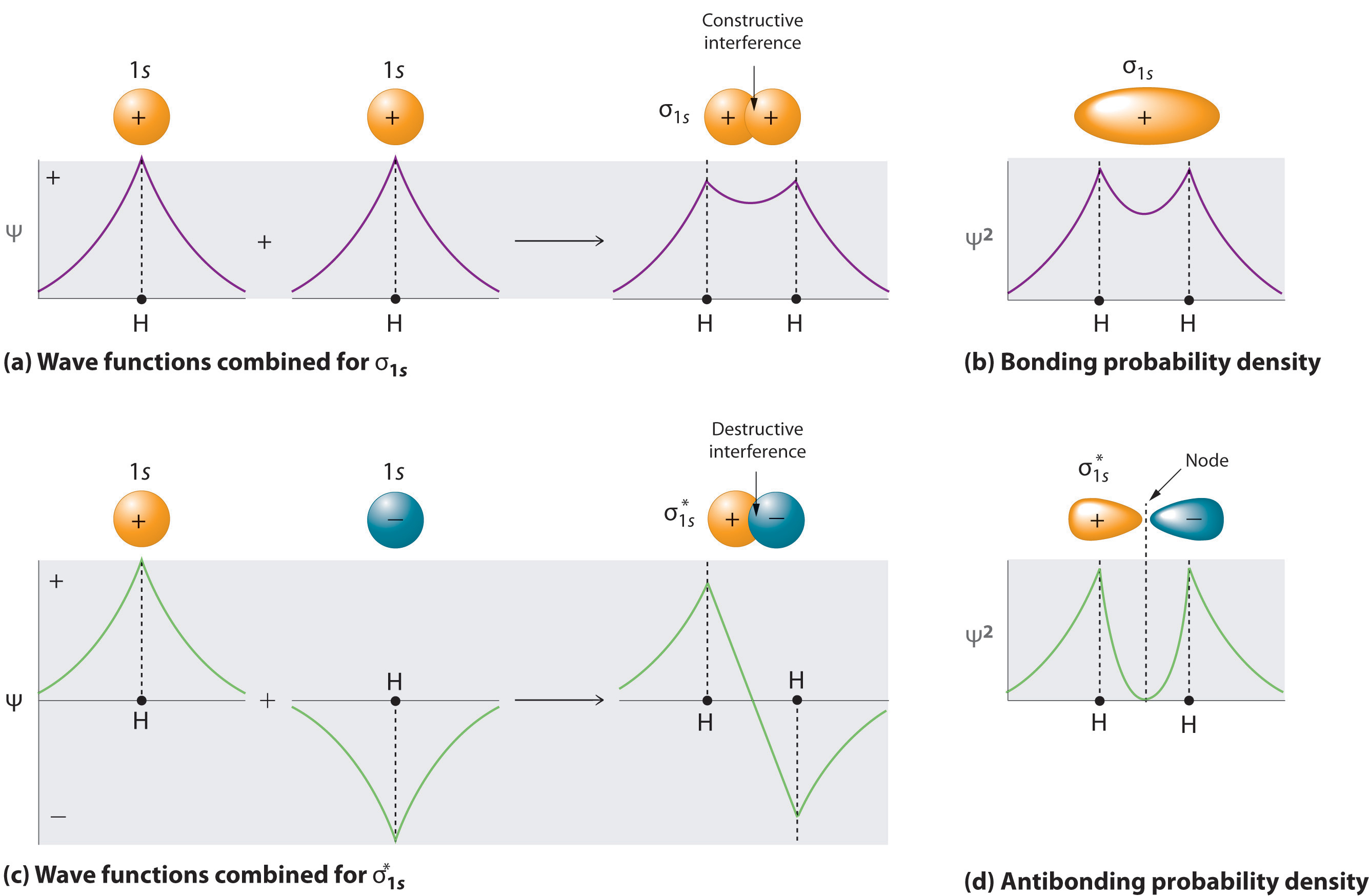
A molecule will have as many molecular orbitals as there are atomic orbitals used in the basis set (\(N\) in Equation \(\ref{9.5.12}\)). Adding two atomic orbitals corresponds to constructive interference between two waves, thus reinforcing their intensity; the internuclear electron probability density is increased. The molecular orbital corresponding to the sum of the two H 1s orbitals is called a σ1s combination (parts (a) and (b) of Figure 9.5.1 ).

In the sigma (\(σ\)) orbital, the electron density along the internuclear axis and between the nuclei has cylindrical symmetry; that is, all cross-sections perpendicular to the internuclear axis are circles. The subscript 1s denotes the atomic orbitals from which the molecular orbital was derived.
\[ | \sigma _{1s} \rangle = \dfrac{1}{\sqrt{2(1 + S )}} \left( | 1s_A \rangle + | 1s_B \rangle \right) \label{9.7.2} \]
Conversely, subtracting one atomic orbital from another corresponds to destructive interference between two waves, which reduces their intensity and causes a decrease in the internuclear electron probability density (part (c) and part (d) in Figure 9.5.1 ). The resulting pattern contains a node where the electron density is zero. The molecular orbital corresponding to the difference is called \( \sigma _{1s}^{*} \) and has a region of zero electron probability, a nodal plane, perpendicular to the internuclear axis:
\[ | \sigma _{1s}^* \rangle = \dfrac{1}{\sqrt{2(1 - S )}} \left( | 1s_A \rangle - | 1s_B \rangle \right) \label{9.7.3} \]
The electron density in the σ1s molecular orbital is greatest between the two positively charged nuclei, and the resulting electron–nucleus electrostatic attractions reduce repulsions between the nuclei. Thus the σ1s orbital represents a bonding molecular orbital. A molecular orbital that forms when atomic orbitals or orbital lobes with the same sign interact to give increased electron probability between the nuclei due to constructive reinforcement of the wavefunctions. In contrast, electrons in the \( \sigma _{1s}^{\star } \) orbital are generally found in the space outside the internuclear region. Because this allows the positively charged nuclei to repel one another, the \( \sigma _{1s}^{\star } \) orbital is an antibonding molecular orbital (a molecular orbital that forms when atomic orbitals or orbital lobes of opposite sign interact to give decreased electron probability between the nuclei due to destructive reinforcement of the wavefunctions).
Antibonding orbitals contain a node perpendicular to the internuclear axis; bonding orbitals do not.
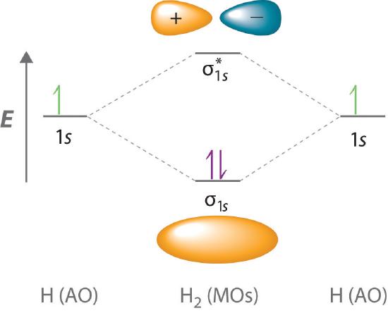
Because electrons in the σ1s orbital interact simultaneously with both nuclei, they have a lower energy than electrons that interact with only one nucleus. This means that the σ1s molecular orbital has a lower energy than either of the hydrogen 1s atomic orbitals. Conversely, electrons in the \( \sigma _{1s}^{\star } \) orbital interact with only one hydrogen nucleus at a time. In addition, they are farther away from the nucleus than they were in the parent hydrogen 1s atomic orbitals. Consequently, the \( \sigma _{1s}^{\star } \) molecular orbital has a higher energy than either of the hydrogen 1s atomic orbitals. The σ1s (bonding) molecular orbital is stabilized relative to the 1s atomic orbitals, and the \( \sigma _{1s}^{\star } \) (antibonding) molecular orbital is destabilized. The relative energy levels of these orbitals are shown in the energy-level diagram (a schematic drawing that compares the energies of the molecular orbitals (bonding, antibonding, and nonbonding) with the energies of the parent atomic orbitals) in Figure 9.5.2

A bonding molecular orbital is always lower in energy (more stable) than the component atomic orbitals, whereas an antibonding molecular orbital is always higher in energy (less stable).
Expanding Beyond the 1s Orbital Basis Set
This picture of bonding in H2+ in the previous section is very simple, but gives reasonable results when compared to an exact calculation. The equilibrium bond distance is 134 pm compared to 106 pm (exact), and a dissociation energy is 1.8 eV compared to 2.8 eV (exact). To better describe chemical bonding we need to account for the increase in electron density between the two nuclei. The 1s orbitals alone are not particularly good for this purpose because they are spherically symmetric and show no preference for the space between the atomic nuclei. The use of additional atomic orbitals can correct this situation and provide additional parameters, which can be optimized by the linear variational method, to give a better function with a lower energy and more accurate description of the charge density.
The energy of the non-normalized molecular orbital can be calculated from the expectation value integral of the Hamiltonian,
\[E_{J} = \dfrac{\left \langle \psi _{J} | \hat {H} _{elec} | \psi _{J} \right \rangle}{\left \langle \psi _{J} | \psi _{J} \right \rangle} \label {9.5.13} \]
This is the variational energy using \(| \psi _{J} \rangle\) as the trail wavefunction. After substituting the LCAO expansion for \(| \psi _{J} \rangle\) (Equation \ref{9.5.12}) into the energy expression of Equation \ref{9.5.13} results in:
\[\begin{align} E_{J} &= \dfrac{\left \langle \displaystyle \sum_i c_{J,i}^* \phi_i \right | \hat {H} _{elec} \left | \displaystyle \sum_j c_{J,i} \phi_j \right \rangle}{\left \langle \displaystyle \sum_i c_{J,i}^* \phi_j | \displaystyle \sum_j c_{J,j} \phi_j\right \rangle} \label {9.5.14} \\[4pt] &= \dfrac{ \displaystyle \sum_{i,j} c_{J,i}^* c_{J,j} \left \langle \phi_i \right| \hat {H} _{elec} \left| \phi_j \right \rangle}{ \displaystyle\sum_{i,j} c_{J,i}^* c_{J,j} \left \langle \phi_i | \phi_j\right \rangle} \label {9.5.15} \\[4pt] &= \dfrac{ \displaystyle \sum_{i,j} c_{J,i}^* c_{J,j} H_{ij}}{ \displaystyle \sum_{i,j} c_{J,i}^* c_{J,j} S_{ij} } \label {9.5.16} \end{align} \]
where \(H_{ij}\) is the Hamiltonian matrix element.
\[H_{ij} = \langle \phi_i | \hat {H} _{elec} | \phi_j \rangle \nonumber \]
Following the variational theorem, to determine the coefficients of the LCAO expansion \(c_i\), we need to minimize \(E_J\)
\[ \dfrac{\partial E_J}{\partial c_k} = 0 \label{9.5.17} \]
for all \(k\). This requires solving \(N\) linear equations to hold true (where \(N\) is the number of atomic orbitals in the basis)
\[ \sum_{i=1}^{N} c_i (H_{ki} - ES_{ki}) = 0 \label{9.5.18} \]
These equations are the secular equations and were discussed previously in the context of the linear variational method approximation. For the two basis set expansion (\(N\)) in Figure 9.5.1 , these are
\[\begin{array}{rcl} c_1(H_{11} - ES_{11}) + c_2(H_{12} - ES_{12}) & = & 0 \\ c_1(H_{12} - ES_{12}) + c_2(H_{22} - ES_{22}) & = & 0 \end{array} \label{9.5.19} \]
where \(c_1\) and \(c_2\) are the coefficients in the linear combination of the atomic orbitals used to construct the molecular orbital. Writing this set of homogeneous linear equations in matrix form gives
\[\begin{pmatrix} H_{11} - ES_{11} & H_{12} - ES_{12} \\ H_{12} - ES_{12} & H_{22} - ES_{22} \end{pmatrix} \begin{pmatrix} c_1 \\ c_2 \end{pmatrix} = \begin{pmatrix} 0 \\ 0 \end{pmatrix} \label{9.5.20} \]
Solving these secular equations with N different atomic orbitals in the expansion (Equation \(\ref{9.5.12}\)) requires finding the N roots of an N order polynomial.
\[\left|\begin{array}{lcc} H_{11} - ES_{11} & H_{12} - ES_{12} & \ldots\\ H_{12} - ES_{12} & H_{22} - ES_{22} &\ldots \\ \ldots &\ldots &\ldots \end{array}\right|=0\label{23} \]
Each molecular orbital (\(| \psi_J \rangle\)) from this treatment has an energy \(E_J\) that is given by a different set of coefficients, \(\{c_{ij}\}\) where \(i\) runs over all \(N\) functions in the basis (i.e., number of the atomic orbitals in the LCAO approximation of Equation \(\ref{9.5.12}\)), and \(J\) runs over molecular orbitals. Solve the set of linear equations using that specific \(E_J\) to determine \(c_{ij}\) values.
- Select a set of N basis functions
- Determine all N( N –1)/2 values of both \(H_{ij}\) and \(S_{ij}\)
- Form the secular determinant; determine N roots \(E_j\) of secular equation
- For each \(E_J\) solve the set of linear equations to determine the basis set coefficients \(c_{ij\}) for the j-th molecular orbital
For more information on solving the Secular equations check here.
The greater the number of atomic orbitals \(N\) that combine to genera the molecular orbitals (Equation \(\ref{9.5.12}\)), the more accurate the LCAO approximation is. This is expected based on our discussions of the variational method examples. Hence, the \(\psi_+\) and \(\psi_-\) molecular orbitals for \(H_2^+\) are better expressed with higher energy hydrogenic wavefunctions
\[| \psi_J \rangle = c_{J,1} 1s_A + c_{J,2} 1s_B + c_{J,3} 2s_A + c_{J,4} 2s_B + c_{J,5} 2p_{z,A} + c_{J,6} 2p_{z,B} \label{9.5.24} \]
The reasons that only the \(p_z\) atomic orbitals are included in this expansion are discussed later.
Contributors and Attributions
David M. Hanson, Erica Harvey, Robert Sweeney, Theresa Julia Zielinski ("Quantum States of Atoms and Molecules")

