2.5: A Vibrating Membrane
- Page ID
- 13379
\( \newcommand{\vecs}[1]{\overset { \scriptstyle \rightharpoonup} {\mathbf{#1}} } \)
\( \newcommand{\vecd}[1]{\overset{-\!-\!\rightharpoonup}{\vphantom{a}\smash {#1}}} \)
\( \newcommand{\id}{\mathrm{id}}\) \( \newcommand{\Span}{\mathrm{span}}\)
( \newcommand{\kernel}{\mathrm{null}\,}\) \( \newcommand{\range}{\mathrm{range}\,}\)
\( \newcommand{\RealPart}{\mathrm{Re}}\) \( \newcommand{\ImaginaryPart}{\mathrm{Im}}\)
\( \newcommand{\Argument}{\mathrm{Arg}}\) \( \newcommand{\norm}[1]{\| #1 \|}\)
\( \newcommand{\inner}[2]{\langle #1, #2 \rangle}\)
\( \newcommand{\Span}{\mathrm{span}}\)
\( \newcommand{\id}{\mathrm{id}}\)
\( \newcommand{\Span}{\mathrm{span}}\)
\( \newcommand{\kernel}{\mathrm{null}\,}\)
\( \newcommand{\range}{\mathrm{range}\,}\)
\( \newcommand{\RealPart}{\mathrm{Re}}\)
\( \newcommand{\ImaginaryPart}{\mathrm{Im}}\)
\( \newcommand{\Argument}{\mathrm{Arg}}\)
\( \newcommand{\norm}[1]{\| #1 \|}\)
\( \newcommand{\inner}[2]{\langle #1, #2 \rangle}\)
\( \newcommand{\Span}{\mathrm{span}}\) \( \newcommand{\AA}{\unicode[.8,0]{x212B}}\)
\( \newcommand{\vectorA}[1]{\vec{#1}} % arrow\)
\( \newcommand{\vectorAt}[1]{\vec{\text{#1}}} % arrow\)
\( \newcommand{\vectorB}[1]{\overset { \scriptstyle \rightharpoonup} {\mathbf{#1}} } \)
\( \newcommand{\vectorC}[1]{\textbf{#1}} \)
\( \newcommand{\vectorD}[1]{\overrightarrow{#1}} \)
\( \newcommand{\vectorDt}[1]{\overrightarrow{\text{#1}}} \)
\( \newcommand{\vectE}[1]{\overset{-\!-\!\rightharpoonup}{\vphantom{a}\smash{\mathbf {#1}}}} \)
\( \newcommand{\vecs}[1]{\overset { \scriptstyle \rightharpoonup} {\mathbf{#1}} } \)
\( \newcommand{\vecd}[1]{\overset{-\!-\!\rightharpoonup}{\vphantom{a}\smash {#1}}} \)
\(\newcommand{\avec}{\mathbf a}\) \(\newcommand{\bvec}{\mathbf b}\) \(\newcommand{\cvec}{\mathbf c}\) \(\newcommand{\dvec}{\mathbf d}\) \(\newcommand{\dtil}{\widetilde{\mathbf d}}\) \(\newcommand{\evec}{\mathbf e}\) \(\newcommand{\fvec}{\mathbf f}\) \(\newcommand{\nvec}{\mathbf n}\) \(\newcommand{\pvec}{\mathbf p}\) \(\newcommand{\qvec}{\mathbf q}\) \(\newcommand{\svec}{\mathbf s}\) \(\newcommand{\tvec}{\mathbf t}\) \(\newcommand{\uvec}{\mathbf u}\) \(\newcommand{\vvec}{\mathbf v}\) \(\newcommand{\wvec}{\mathbf w}\) \(\newcommand{\xvec}{\mathbf x}\) \(\newcommand{\yvec}{\mathbf y}\) \(\newcommand{\zvec}{\mathbf z}\) \(\newcommand{\rvec}{\mathbf r}\) \(\newcommand{\mvec}{\mathbf m}\) \(\newcommand{\zerovec}{\mathbf 0}\) \(\newcommand{\onevec}{\mathbf 1}\) \(\newcommand{\real}{\mathbb R}\) \(\newcommand{\twovec}[2]{\left[\begin{array}{r}#1 \\ #2 \end{array}\right]}\) \(\newcommand{\ctwovec}[2]{\left[\begin{array}{c}#1 \\ #2 \end{array}\right]}\) \(\newcommand{\threevec}[3]{\left[\begin{array}{r}#1 \\ #2 \\ #3 \end{array}\right]}\) \(\newcommand{\cthreevec}[3]{\left[\begin{array}{c}#1 \\ #2 \\ #3 \end{array}\right]}\) \(\newcommand{\fourvec}[4]{\left[\begin{array}{r}#1 \\ #2 \\ #3 \\ #4 \end{array}\right]}\) \(\newcommand{\cfourvec}[4]{\left[\begin{array}{c}#1 \\ #2 \\ #3 \\ #4 \end{array}\right]}\) \(\newcommand{\fivevec}[5]{\left[\begin{array}{r}#1 \\ #2 \\ #3 \\ #4 \\ #5 \\ \end{array}\right]}\) \(\newcommand{\cfivevec}[5]{\left[\begin{array}{c}#1 \\ #2 \\ #3 \\ #4 \\ #5 \\ \end{array}\right]}\) \(\newcommand{\mattwo}[4]{\left[\begin{array}{rr}#1 \amp #2 \\ #3 \amp #4 \\ \end{array}\right]}\) \(\newcommand{\laspan}[1]{\text{Span}\{#1\}}\) \(\newcommand{\bcal}{\cal B}\) \(\newcommand{\ccal}{\cal C}\) \(\newcommand{\scal}{\cal S}\) \(\newcommand{\wcal}{\cal W}\) \(\newcommand{\ecal}{\cal E}\) \(\newcommand{\coords}[2]{\left\{#1\right\}_{#2}}\) \(\newcommand{\gray}[1]{\color{gray}{#1}}\) \(\newcommand{\lgray}[1]{\color{lightgray}{#1}}\) \(\newcommand{\rank}{\operatorname{rank}}\) \(\newcommand{\row}{\text{Row}}\) \(\newcommand{\col}{\text{Col}}\) \(\renewcommand{\row}{\text{Row}}\) \(\newcommand{\nul}{\text{Nul}}\) \(\newcommand{\var}{\text{Var}}\) \(\newcommand{\corr}{\text{corr}}\) \(\newcommand{\len}[1]{\left|#1\right|}\) \(\newcommand{\bbar}{\overline{\bvec}}\) \(\newcommand{\bhat}{\widehat{\bvec}}\) \(\newcommand{\bperp}{\bvec^\perp}\) \(\newcommand{\xhat}{\widehat{\xvec}}\) \(\newcommand{\vhat}{\widehat{\vvec}}\) \(\newcommand{\uhat}{\widehat{\uvec}}\) \(\newcommand{\what}{\widehat{\wvec}}\) \(\newcommand{\Sighat}{\widehat{\Sigma}}\) \(\newcommand{\lt}{<}\) \(\newcommand{\gt}{>}\) \(\newcommand{\amp}{&}\) \(\definecolor{fillinmathshade}{gray}{0.9}\)- To apply the wave equations to a two-dimensional membrane (rectangles and circles)
- To recognize the possible geometries of a nodes in two-dimensional systems
So far, we’ve looked at waves in one dimension, traveling along a string or sound waves going down a narrow tube. However, waves in higher dimensions than one are very familiar—water waves on the surface of a pond, or sound waves moving out from a source in three dimensions. It is pleasant to find that these waves in higher dimensions satisfy wave equations which are a very natural extension of the one we found for a string, and—very important—they also satisfy the Principle of Superposition, in other words, if waves meet, you just add the contribution from each wave. In the next two paragraphs, we go into more detail, but this Principle of Superposition is the crucial lesson.
The Wave Equation and Superposition in More Dimensions
What happens in higher dimensions? Let’s consider two dimensions, for example waves in an elastic sheet like a drumhead. If the rest position for the elastic sheet is the (\(x\), \(y\)) plane, so when it’s vibrating it’s moving up and down in the z-direction, its configuration at any instant of time is a function. \(u(x,y,t)\)
In fact, we could do the same thing we did for the string, looking at the total forces on a little bit and applying Newton’s Second Law. In this case that would mean taking one little bit of the drumhead, and instead of a small stretch of string with tension pulling the two ends, we would have a small square of the elastic sheet, with tension pulling all around the edge. Remember that the net force on the bit of string came about because the string was curving around, so the tensions at the opposite ends tugged in slightly different directions, and did not cancel. The \(\frac{\partial^2}{\partial x^2}\) term measured that curvature, the rate of change of slope. In two dimensions, thinking of a small square of the elastic sheet, things are more complicated. Visualize the bit of sheet to be momentarily like a tiny patch on a balloon, you’ll see it curves in two directions, and tension forces must be tugging all around the edges. The total force on the little square comes about because the tension forces on opposite sides are out of line if the surface is curving around, now we have to add two sets of almost-opposite forces from the two pairs of sides. The math is now shown here, but it is at least plausible that the equation is:
\[ \dfrac{ \partial^2 u(x,y,t)}{\partial x^2} + \dfrac{ \partial^2 u(x,y,t)}{\partial y^2} = \dfrac{1}{v^2} \dfrac{ \partial^2 u(x,y,t)}{\partial t^2} \label{2.5.1} \]
The physics of this equation is that the acceleration of a tiny bit of the sheet comes from out-of-balance tensions caused by the sheet curving around in both the x- and y-directions, this is why there are the two terms on the left hand side.
And, going to three dimensions is easy: add one more term to give
\[ \dfrac{ \partial^2 u(x,y,,z,t)}{\partial x^2} + \dfrac{ \partial^2 u(x,y,z,t)}{\partial y^2} + \dfrac{ \partial^2 u(x,y,z,t)}{\partial z^2} = \dfrac{1}{v^2} \dfrac{ \partial^2 u(x,y,z,t)}{\partial t^2} \label{2.5.2} \]
This sum of partial differentiations in space is so common in physics that there’s a shorthand:
\[ \nabla^2 = \left( \dfrac{ \partial^2}{\partial x^2}, \dfrac{ \partial^2}{\partial y^2}, \dfrac{ \partial^2}{\partial z^2} \right) \nonumber \]
so Equation \ref{2.5.2} can be more easily written as
\[ \nabla^2 u(x,y,z,t) = \dfrac{1}{v^2} \dfrac{\partial^2 u(x,y,z,t)}{\partial t^2} \nonumber \]
Just as we found in one dimension traveling harmonic waves (no boundary conditions)
\[u(x,t) = A \sin (kx -\omega t) \nonumber \]
with \(\omega=\nu k \), you can verify that the three-dimensional equation has harmonic solutions
\[u(x,y,z,t) = A \sin (k_x x +k_x +k_z z -\omega t) \nonumber \]
with \(\omega = \nu |\vec{k|}\) where \(|k| = \sqrt{k_x^2+k_y^2+k_z^2}\).
\(\vec{k}\) is a vector in the direction the wave is moving. The electric and magnetic fields in a radio wave or light wave have just this form (or, closer to the source, a very similar equivalent expression for outgoing spheres of waves, rather than plane waves).
It’s important to realize that the 2D wave equation (Equation \ref{2.5.1}) is still a linear equation, so the Principle of Superposition still holds. If two waves on an elastic sheet, or the surface of a pond, meet each other, the result at any point is given by simply adding the displacements from the individual waves. We’ll begin by thinking about waves propagating freely in two and three dimensions, than later consider waves in restricted areas, such as a drum head.
Vibrational Modes of a Rectangular Membrane
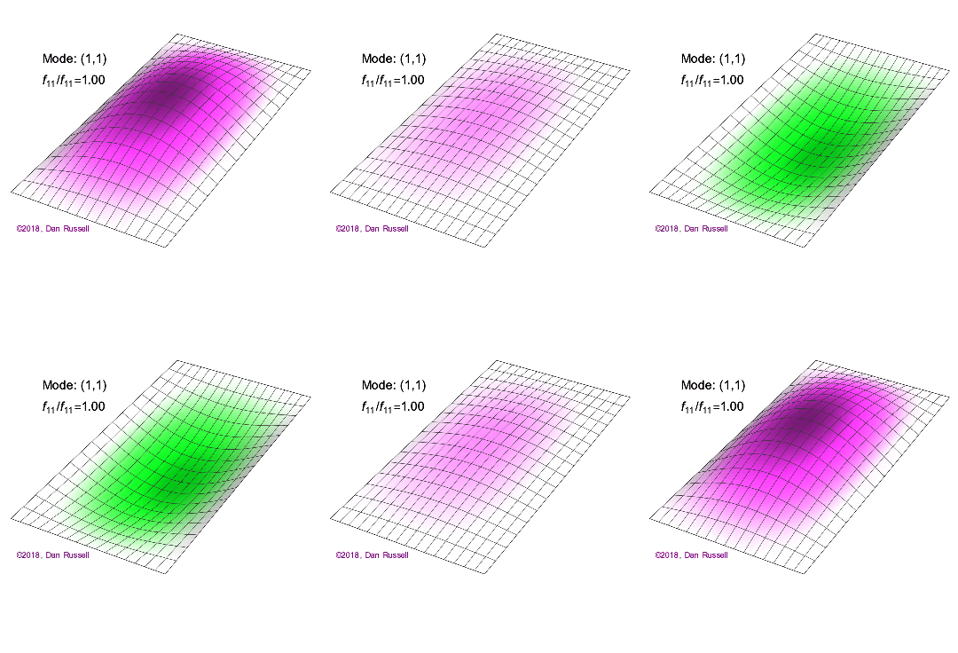
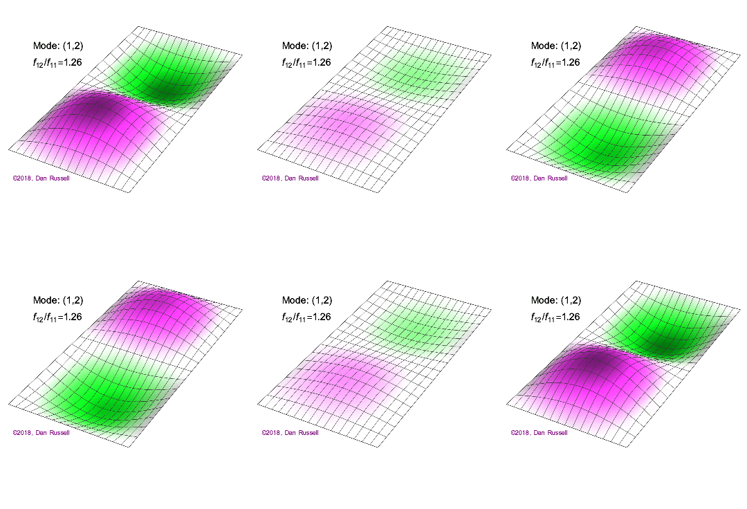
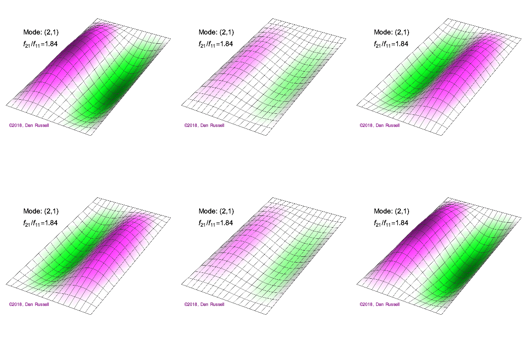
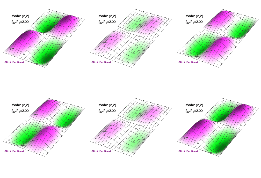
A one-dimensional wave does not have a choice in how it propagates: it just moves along the line (well, it could get partly reflected by some change in the line and part of it go backwards). However, when we go to higher dimensions, how a wave disturbance starting in some localized region spreads out is far from obvious. But we can begin by recalling some simple cases: dropping a pebble into still water causes an outward moving circle of ripples. If we grant that light is a wave, we notice a beam of light changes direction on going from air into glass. Of course, it is not immediately evident that light is a wave: we’ll talk a lot more about that later. A few solutions (both temporal and spatials) are shown below together with their quantum numbers (\(n_x\) and \(n_y\)).
Solving for the function \(u(x,y,t)\) in a vibrating, rectangular membrane is done in a similar fashion by separation of variables, and setting boundary conditions. The solved function is very similar, where
\[u(x,y,t) = A_{nm} \cos(\omega_{nm} t + \phi_{nm}) \sin \left(\dfrac {n_x \pi x}{a}\right) \sin\left(\dfrac {n_y\pi y}{b}\right) \label{2.5.6b} \]
where
- \(a\) is the length of the rectangular membrane and \(b\) is the width, and
- \(n_x\) and \(n_y\) are two quantum numbers (one in each dimension).
As with the solutions to 1-D wave equations, a node is a point (or line) on a structure that does not move while the rest of the structure is vibrating.
For the following 2-D solutions in Figure 2.5.1 , how many nodes are there, what is the geometry and how would you characterize them?
- (\(n_x=1\), \(n_y=1\)
- (\(n_x=2\), \(n_y=1\)
Solution
a. The (\(n_x=1\), \(n_y=1\) solution in Figure 2.5.1 has zero nodes. That is, no spot in the membrane (other than the boundaries) is not moving during the motion of the membrane.
b. The (\(n_x=2\), \(n_y=1\) solution in Figure 2.5.1 has one node. It is a line at half the length of the x direction and extends over the entire length of the y direction.
For the (\(n_x=2\), \(n_y=2\) solution to a rectangular membrane in Figure 2.5.1 : how many nodes are there, what is the geometry and how would you characterize them?
- Answer
-
There are two nodes. They are lines and one is at half the length of the x direction and extends over the entire length of the y direction and one if and one is at half the length of the y direction and extends over the entire length of the x direction
Vibrational Modes of a Circular Membrane
The basic principles of a vibrating rectangular membrane applies to other 2-D members including circular membranes. However, the mathematics and solutions are a bit more complicated. The solutions are best represented in polar notation (instead of rectangular like in Equation \ref{2.5.6b}) and have the following functional form
\[u(r, \theta, t)=J_{m}\left(\lambda_{m n} r\right) \cos m \theta \cos c \lambda_{m n} t \nonumber \]
where \(J_m\) are Bessel functions (these are oscillatory functions) and \(\lambda\) are constants. This system has two quantum numbers (\(m\) and \(n\)) that serve the same function as \(n_x\) and \(n_y\) do in the rectangular membranes. In the animations in Figure 2.5.2 , the nodal diameters and circles show up as white regions that do not oscillate, while the red and blue regions indicate positive and negative displacements.
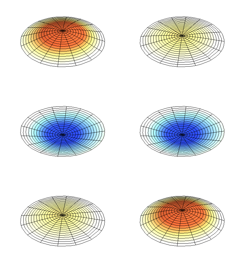
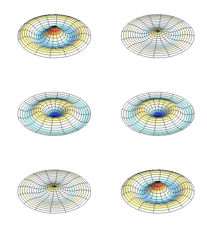
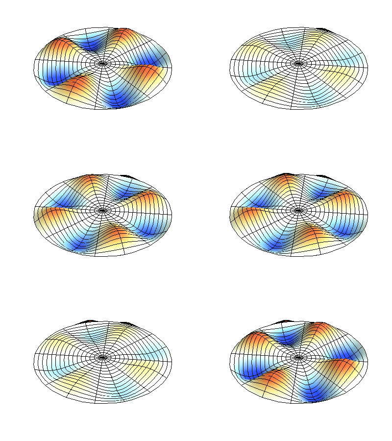
Figure 2.5.2 (left) shows the fundamental mode shape for a vibrating circular membrane, while the other two modes are excited modes with more complex nodal character.
How many nodes are there in the three solutions for a circular membrane in Figure 2.5.2 , what are their geometries, and how would you characterize them?
- Answer
-
(left) zero nodes
(middle) two nodes. They are circular at approximately 1/3 and 2/3 the radius (these are radial nodes = at fixed radii)
(right) four nodes. They are lines at 45° angle from the center (these are angular nodes = at fixed angles).

