
15.6: Orthogonal Matrices
- Page ID
- 106901

\( \newcommand{\vecs}[1]{\overset { \scriptstyle \rightharpoonup} {\mathbf{#1}} } \)
\( \newcommand{\vecd}[1]{\overset{-\!-\!\rightharpoonup}{\vphantom{a}\smash {#1}}} \)
\( \newcommand{\id}{\mathrm{id}}\) \( \newcommand{\Span}{\mathrm{span}}\)
( \newcommand{\kernel}{\mathrm{null}\,}\) \( \newcommand{\range}{\mathrm{range}\,}\)
\( \newcommand{\RealPart}{\mathrm{Re}}\) \( \newcommand{\ImaginaryPart}{\mathrm{Im}}\)
\( \newcommand{\Argument}{\mathrm{Arg}}\) \( \newcommand{\norm}[1]{\| #1 \|}\)
\( \newcommand{\inner}[2]{\langle #1, #2 \rangle}\)
\( \newcommand{\Span}{\mathrm{span}}\)
\( \newcommand{\id}{\mathrm{id}}\)
\( \newcommand{\Span}{\mathrm{span}}\)
\( \newcommand{\kernel}{\mathrm{null}\,}\)
\( \newcommand{\range}{\mathrm{range}\,}\)
\( \newcommand{\RealPart}{\mathrm{Re}}\)
\( \newcommand{\ImaginaryPart}{\mathrm{Im}}\)
\( \newcommand{\Argument}{\mathrm{Arg}}\)
\( \newcommand{\norm}[1]{\| #1 \|}\)
\( \newcommand{\inner}[2]{\langle #1, #2 \rangle}\)
\( \newcommand{\Span}{\mathrm{span}}\) \( \newcommand{\AA}{\unicode[.8,0]{x212B}}\)
\( \newcommand{\vectorA}[1]{\vec{#1}} % arrow\)
\( \newcommand{\vectorAt}[1]{\vec{\text{#1}}} % arrow\)
\( \newcommand{\vectorB}[1]{\overset { \scriptstyle \rightharpoonup} {\mathbf{#1}} } \)
\( \newcommand{\vectorC}[1]{\textbf{#1}} \)
\( \newcommand{\vectorD}[1]{\overrightarrow{#1}} \)
\( \newcommand{\vectorDt}[1]{\overrightarrow{\text{#1}}} \)
\( \newcommand{\vectE}[1]{\overset{-\!-\!\rightharpoonup}{\vphantom{a}\smash{\mathbf {#1}}}} \)
\( \newcommand{\vecs}[1]{\overset { \scriptstyle \rightharpoonup} {\mathbf{#1}} } \)
\( \newcommand{\vecd}[1]{\overset{-\!-\!\rightharpoonup}{\vphantom{a}\smash {#1}}} \)
\(\newcommand{\avec}{\mathbf a}\) \(\newcommand{\bvec}{\mathbf b}\) \(\newcommand{\cvec}{\mathbf c}\) \(\newcommand{\dvec}{\mathbf d}\) \(\newcommand{\dtil}{\widetilde{\mathbf d}}\) \(\newcommand{\evec}{\mathbf e}\) \(\newcommand{\fvec}{\mathbf f}\) \(\newcommand{\nvec}{\mathbf n}\) \(\newcommand{\pvec}{\mathbf p}\) \(\newcommand{\qvec}{\mathbf q}\) \(\newcommand{\svec}{\mathbf s}\) \(\newcommand{\tvec}{\mathbf t}\) \(\newcommand{\uvec}{\mathbf u}\) \(\newcommand{\vvec}{\mathbf v}\) \(\newcommand{\wvec}{\mathbf w}\) \(\newcommand{\xvec}{\mathbf x}\) \(\newcommand{\yvec}{\mathbf y}\) \(\newcommand{\zvec}{\mathbf z}\) \(\newcommand{\rvec}{\mathbf r}\) \(\newcommand{\mvec}{\mathbf m}\) \(\newcommand{\zerovec}{\mathbf 0}\) \(\newcommand{\onevec}{\mathbf 1}\) \(\newcommand{\real}{\mathbb R}\) \(\newcommand{\twovec}[2]{\left[\begin{array}{r}#1 \\ #2 \end{array}\right]}\) \(\newcommand{\ctwovec}[2]{\left[\begin{array}{c}#1 \\ #2 \end{array}\right]}\) \(\newcommand{\threevec}[3]{\left[\begin{array}{r}#1 \\ #2 \\ #3 \end{array}\right]}\) \(\newcommand{\cthreevec}[3]{\left[\begin{array}{c}#1 \\ #2 \\ #3 \end{array}\right]}\) \(\newcommand{\fourvec}[4]{\left[\begin{array}{r}#1 \\ #2 \\ #3 \\ #4 \end{array}\right]}\) \(\newcommand{\cfourvec}[4]{\left[\begin{array}{c}#1 \\ #2 \\ #3 \\ #4 \end{array}\right]}\) \(\newcommand{\fivevec}[5]{\left[\begin{array}{r}#1 \\ #2 \\ #3 \\ #4 \\ #5 \\ \end{array}\right]}\) \(\newcommand{\cfivevec}[5]{\left[\begin{array}{c}#1 \\ #2 \\ #3 \\ #4 \\ #5 \\ \end{array}\right]}\) \(\newcommand{\mattwo}[4]{\left[\begin{array}{rr}#1 \amp #2 \\ #3 \amp #4 \\ \end{array}\right]}\) \(\newcommand{\laspan}[1]{\text{Span}\{#1\}}\) \(\newcommand{\bcal}{\cal B}\) \(\newcommand{\ccal}{\cal C}\) \(\newcommand{\scal}{\cal S}\) \(\newcommand{\wcal}{\cal W}\) \(\newcommand{\ecal}{\cal E}\) \(\newcommand{\coords}[2]{\left\{#1\right\}_{#2}}\) \(\newcommand{\gray}[1]{\color{gray}{#1}}\) \(\newcommand{\lgray}[1]{\color{lightgray}{#1}}\) \(\newcommand{\rank}{\operatorname{rank}}\) \(\newcommand{\row}{\text{Row}}\) \(\newcommand{\col}{\text{Col}}\) \(\renewcommand{\row}{\text{Row}}\) \(\newcommand{\nul}{\text{Nul}}\) \(\newcommand{\var}{\text{Var}}\) \(\newcommand{\corr}{\text{corr}}\) \(\newcommand{\len}[1]{\left|#1\right|}\) \(\newcommand{\bbar}{\overline{\bvec}}\) \(\newcommand{\bhat}{\widehat{\bvec}}\) \(\newcommand{\bperp}{\bvec^\perp}\) \(\newcommand{\xhat}{\widehat{\xvec}}\) \(\newcommand{\vhat}{\widehat{\vvec}}\) \(\newcommand{\uhat}{\widehat{\uvec}}\) \(\newcommand{\what}{\widehat{\wvec}}\) \(\newcommand{\Sighat}{\widehat{\Sigma}}\) \(\newcommand{\lt}{<}\) \(\newcommand{\gt}{>}\) \(\newcommand{\amp}{&}\) \(\definecolor{fillinmathshade}{gray}{0.9}\)A nonsingular matrix is called orthogonal when its inverse is equal to its transpose:
\[\mathbf{A}^T =\mathbf{A}^{-1}\rightarrow \mathbf{A}^T\mathbf{A} = \mathbf{I}. \nonumber \]
For example, for the matrix
\[\mathbf{A}=\begin{pmatrix} \cos \theta&-\sin \theta \\ \sin \theta&\cos \theta \end{pmatrix}, \nonumber \]
the inverse is
\[ \mathbf{A}^{-1} =\begin{pmatrix} \cos \theta&\sin \theta \\ -\sin \theta&\cos \theta \end{pmatrix} =\mathbf{A}^T \nonumber \]
We do not need to calculate the inverse to see if the matrix is orthogonal. We can transpose the matrix, multiply the result by the matrix, and see if we get the identity matrix as a result:
\[\mathbf{A}^T=\begin{pmatrix} \cos \theta&\sin \theta \\ -\sin \theta&\cos \theta \end{pmatrix} \nonumber \]
\[ \mathbf{A}^T \mathbf{A} =\begin{pmatrix} \cos \theta&\sin \theta \\ -\sin \theta&\cos \theta \end{pmatrix}\begin{pmatrix} \cos \theta&-\sin \theta \\ \sin \theta&\cos \theta \end{pmatrix} =\begin{pmatrix} (\cos^2 \theta+ \sin^2\theta)&0 \\ 0&(\sin^2 \theta+ \cos^2\theta) \end{pmatrix} =\begin{pmatrix} 1&0 \\ 0&1 \end{pmatrix} \nonumber \]
The columns of orthogonal matrices form a system of orthonormal vectors (Section 14.2):
\[\mathbf{M}=\begin{pmatrix} a_1&b_1&c_1 \\ a_2&b_2&c_2 \\ a_3&b_3&c_3 \end{pmatrix}\rightarrow \mathbf{a}=\begin{pmatrix}a_1\\a_2\\a_3\end{pmatrix}; \;\mathbf{b}=\begin{pmatrix}b_1\\b_2\\b_3\end{pmatrix}; \;\mathbf{c}=\begin{pmatrix}c_1\\c_2\\c_3\end{pmatrix} \nonumber \]
\[\mathbf{a}\cdot\mathbf{b}=\mathbf{a}\cdot\mathbf{c}=\mathbf{c}\cdot\mathbf{b}=0 \nonumber \]
\[|\mathbf{a}|=|\mathbf{b}|=|\mathbf{c}|=1 \nonumber \]
Prove that the matrix \(\mathbf{M}\) is an orthogonal matrix and show that its columns form a set of orthonormal vectors.
\[\mathbf{M}=\begin{pmatrix} 2/3&1/3&-2/3 \\ 2/3&-2/3&1/3 \\ 1/3&2/3&2/3 \end{pmatrix} \nonumber \]
Note: This problem is also available in video format: http://tinyurl.com/k2tkny5
Solution
We first need to prove that \(\mathbf{M}^T\mathbf{M}=1\)
\[\mathbf{M}=\begin{pmatrix} {\color{red}2/3}&{\color{blue}1/3}&-2/3 \\ {\color{red}2/3}&{\color{blue}-2/3}&1/3 \\ {\color{red}1/3}&{\color{blue}2/3}&2/3 \end{pmatrix}\rightarrow \mathbf{M}^T=\begin{pmatrix} {\color{red}2/3}&{\color{red}2/3}&{\color{red}1/3}& \\ {\color{blue}1/3}&{\color{blue}-2/3}&{\color{blue}2/3} \\ -2/3&1/3&2/3 \end{pmatrix} \nonumber \]
\[\mathbf{M}^T\mathbf{M}=\begin{pmatrix} 1&0&0 \\ 0&1&0 \\ 0&0&1 \end{pmatrix}=\mathbf{I} \nonumber \]
Because \(\mathbf{M}^T\mathbf{M}=\mathbf{I}\), the matrix is orthogonal.
We now how to prove that the columns for a set of orthonormal vectors. The vectors are:
\[\mathbf{a}=2/3\mathbf{i}+2/3\mathbf{j}+1/3\mathbf{i}= \begin{pmatrix}2/3\\2/3\\1/3\end{pmatrix}\nonumber \]
\[\mathbf{b}=1/3\mathbf{i}-2/3\mathbf{j}+2/3\mathbf{i}= \begin{pmatrix}1/3\\-2/3\\2/3\end{pmatrix}\nonumber \]
\[\mathbf{c}=-2/3\mathbf{i}+1/3\mathbf{j}+2/3\mathbf{i}= \begin{pmatrix}-2/3\\1/3\\2/3\end{pmatrix}\nonumber \]
The modulii of these vectors are:
\[|\mathbf{a}|^2=(2/3)^2+(2/3)^2+(1/3)^2=1 \nonumber \]
\[|\mathbf{b}|^2=(1/3)^2+(-2/3)^2+(2/3)^2=1 \nonumber \]
\[|\mathbf{c}|^2=(-2/3)^2+(1/3)^2+(2/3)^2=1 \nonumber \]
which proves that the vectors are normalized.
The dot products of the three pairs of vectors are:
\[\mathbf{a}\cdot\mathbf{b}=(2/3)(1/3)+(2/3)(-2/3)+(1/3)(2/3)=0 \nonumber \]
\[\mathbf{a}\cdot\mathbf{c}=(2/3)(-2/3)+(2/3)(1/3)+(1/3)(2/3)=0 \nonumber \]
\[\mathbf{c}\cdot\mathbf{b}=(-2/3)(1/3)+(1/3)(-2/3)+(2/3)(2/3)=0 \nonumber \]
which proves they are mutually orthogonal.
Because the vectors are normalized and mutually orthogonal, they form an orthonormal set.
Orthogonal matrices, when thought as operators that act on vectors, are important because they produce transformations that preserve the lengths of the vectors and the relative angles between them. For example, in two dimensions, the matrix
\[\mathbf{M}_1=1/\sqrt{2}\begin{pmatrix} 1&1 \\ 1&-1 \end{pmatrix} \nonumber \]
is an operator that rotates a vector by \(\pi/4\) in the counterclockwise direction (Figure \(\PageIndex{1}\)) preserving the lengths of the vectors and their relative orientation. In other words, an orthogonal matrix rotates a shape without distorting it. If the columns are orthogonal vectors that are not normalized, as in
\[\mathbf{M}_2=\begin{pmatrix} 1&1 \\ 1&-1 \end{pmatrix}, \nonumber \]
the object changes in size but the shape is not distorted. If, however, the two columns are non-orthogonal vectors, the transformation will distort the shape. Figure \(\PageIndex{1}\) shows an example with the matrix
\[\mathbf{M}_3=\begin{pmatrix} 1&2 \\ -1&1 \end{pmatrix} \nonumber \]
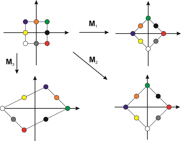
From this discussion, it should not surprise you that all the matrices that represent symmetry operators (Section 15.4) are orthogonal matrices. These operators are used to rotate and reflect the object around different axes and planes without distorting its size and shape.