
15.7: Eigenvalues and Eigenvectors
- Page ID
- 107057

\( \newcommand{\vecs}[1]{\overset { \scriptstyle \rightharpoonup} {\mathbf{#1}} } \)
\( \newcommand{\vecd}[1]{\overset{-\!-\!\rightharpoonup}{\vphantom{a}\smash {#1}}} \)
\( \newcommand{\id}{\mathrm{id}}\) \( \newcommand{\Span}{\mathrm{span}}\)
( \newcommand{\kernel}{\mathrm{null}\,}\) \( \newcommand{\range}{\mathrm{range}\,}\)
\( \newcommand{\RealPart}{\mathrm{Re}}\) \( \newcommand{\ImaginaryPart}{\mathrm{Im}}\)
\( \newcommand{\Argument}{\mathrm{Arg}}\) \( \newcommand{\norm}[1]{\| #1 \|}\)
\( \newcommand{\inner}[2]{\langle #1, #2 \rangle}\)
\( \newcommand{\Span}{\mathrm{span}}\)
\( \newcommand{\id}{\mathrm{id}}\)
\( \newcommand{\Span}{\mathrm{span}}\)
\( \newcommand{\kernel}{\mathrm{null}\,}\)
\( \newcommand{\range}{\mathrm{range}\,}\)
\( \newcommand{\RealPart}{\mathrm{Re}}\)
\( \newcommand{\ImaginaryPart}{\mathrm{Im}}\)
\( \newcommand{\Argument}{\mathrm{Arg}}\)
\( \newcommand{\norm}[1]{\| #1 \|}\)
\( \newcommand{\inner}[2]{\langle #1, #2 \rangle}\)
\( \newcommand{\Span}{\mathrm{span}}\) \( \newcommand{\AA}{\unicode[.8,0]{x212B}}\)
\( \newcommand{\vectorA}[1]{\vec{#1}} % arrow\)
\( \newcommand{\vectorAt}[1]{\vec{\text{#1}}} % arrow\)
\( \newcommand{\vectorB}[1]{\overset { \scriptstyle \rightharpoonup} {\mathbf{#1}} } \)
\( \newcommand{\vectorC}[1]{\textbf{#1}} \)
\( \newcommand{\vectorD}[1]{\overrightarrow{#1}} \)
\( \newcommand{\vectorDt}[1]{\overrightarrow{\text{#1}}} \)
\( \newcommand{\vectE}[1]{\overset{-\!-\!\rightharpoonup}{\vphantom{a}\smash{\mathbf {#1}}}} \)
\( \newcommand{\vecs}[1]{\overset { \scriptstyle \rightharpoonup} {\mathbf{#1}} } \)
\( \newcommand{\vecd}[1]{\overset{-\!-\!\rightharpoonup}{\vphantom{a}\smash {#1}}} \)
\(\newcommand{\avec}{\mathbf a}\) \(\newcommand{\bvec}{\mathbf b}\) \(\newcommand{\cvec}{\mathbf c}\) \(\newcommand{\dvec}{\mathbf d}\) \(\newcommand{\dtil}{\widetilde{\mathbf d}}\) \(\newcommand{\evec}{\mathbf e}\) \(\newcommand{\fvec}{\mathbf f}\) \(\newcommand{\nvec}{\mathbf n}\) \(\newcommand{\pvec}{\mathbf p}\) \(\newcommand{\qvec}{\mathbf q}\) \(\newcommand{\svec}{\mathbf s}\) \(\newcommand{\tvec}{\mathbf t}\) \(\newcommand{\uvec}{\mathbf u}\) \(\newcommand{\vvec}{\mathbf v}\) \(\newcommand{\wvec}{\mathbf w}\) \(\newcommand{\xvec}{\mathbf x}\) \(\newcommand{\yvec}{\mathbf y}\) \(\newcommand{\zvec}{\mathbf z}\) \(\newcommand{\rvec}{\mathbf r}\) \(\newcommand{\mvec}{\mathbf m}\) \(\newcommand{\zerovec}{\mathbf 0}\) \(\newcommand{\onevec}{\mathbf 1}\) \(\newcommand{\real}{\mathbb R}\) \(\newcommand{\twovec}[2]{\left[\begin{array}{r}#1 \\ #2 \end{array}\right]}\) \(\newcommand{\ctwovec}[2]{\left[\begin{array}{c}#1 \\ #2 \end{array}\right]}\) \(\newcommand{\threevec}[3]{\left[\begin{array}{r}#1 \\ #2 \\ #3 \end{array}\right]}\) \(\newcommand{\cthreevec}[3]{\left[\begin{array}{c}#1 \\ #2 \\ #3 \end{array}\right]}\) \(\newcommand{\fourvec}[4]{\left[\begin{array}{r}#1 \\ #2 \\ #3 \\ #4 \end{array}\right]}\) \(\newcommand{\cfourvec}[4]{\left[\begin{array}{c}#1 \\ #2 \\ #3 \\ #4 \end{array}\right]}\) \(\newcommand{\fivevec}[5]{\left[\begin{array}{r}#1 \\ #2 \\ #3 \\ #4 \\ #5 \\ \end{array}\right]}\) \(\newcommand{\cfivevec}[5]{\left[\begin{array}{c}#1 \\ #2 \\ #3 \\ #4 \\ #5 \\ \end{array}\right]}\) \(\newcommand{\mattwo}[4]{\left[\begin{array}{rr}#1 \amp #2 \\ #3 \amp #4 \\ \end{array}\right]}\) \(\newcommand{\laspan}[1]{\text{Span}\{#1\}}\) \(\newcommand{\bcal}{\cal B}\) \(\newcommand{\ccal}{\cal C}\) \(\newcommand{\scal}{\cal S}\) \(\newcommand{\wcal}{\cal W}\) \(\newcommand{\ecal}{\cal E}\) \(\newcommand{\coords}[2]{\left\{#1\right\}_{#2}}\) \(\newcommand{\gray}[1]{\color{gray}{#1}}\) \(\newcommand{\lgray}[1]{\color{lightgray}{#1}}\) \(\newcommand{\rank}{\operatorname{rank}}\) \(\newcommand{\row}{\text{Row}}\) \(\newcommand{\col}{\text{Col}}\) \(\renewcommand{\row}{\text{Row}}\) \(\newcommand{\nul}{\text{Nul}}\) \(\newcommand{\var}{\text{Var}}\) \(\newcommand{\corr}{\text{corr}}\) \(\newcommand{\len}[1]{\left|#1\right|}\) \(\newcommand{\bbar}{\overline{\bvec}}\) \(\newcommand{\bhat}{\widehat{\bvec}}\) \(\newcommand{\bperp}{\bvec^\perp}\) \(\newcommand{\xhat}{\widehat{\xvec}}\) \(\newcommand{\vhat}{\widehat{\vvec}}\) \(\newcommand{\uhat}{\widehat{\uvec}}\) \(\newcommand{\what}{\widehat{\wvec}}\) \(\newcommand{\Sighat}{\widehat{\Sigma}}\) \(\newcommand{\lt}{<}\) \(\newcommand{\gt}{>}\) \(\newcommand{\amp}{&}\) \(\definecolor{fillinmathshade}{gray}{0.9}\)Since square matrices are operators, it should not surprise you that we can determine its eigenvalues and eigenvectors. The eigenvectors are analogous to the eigenfunctions we discussed in Chapter 11.
If \(\mathbf{A}\) is an \(n\times n\) matrix, then a nonzero vector \(\mathbf{x}\) is called an eigenvector of \(\mathbf{A}\) if \(\mathbf{Ax}\) is a scalar multiple of \(\mathbf{x}\):
\[\mathbf{A}\mathbf{x}=\lambda \mathbf{x} \nonumber \]
The scalar \(\lambda\) is called the eigenvalue of \(\mathbf{A}\), and \(\mathbf{x}\) is said to be an eigenvector. For example, the vector \((2,0)\) is an eigenvector of
\[\mathbf{A}=\begin{pmatrix} -2&0 \\ 0&1 \end{pmatrix} \nonumber \]
with eigenvalue \(\lambda=-2\):
\[\begin{pmatrix} -2&0 \\ 0&1 \end{pmatrix}\begin{pmatrix} 2\\ 0 \end{pmatrix}=-2\begin{pmatrix} 2\\ 0 \end{pmatrix} \nonumber \]
Notice that the matrix \(\mathbf{A}\), like any other \(2\times 2\) matrix, transforms a 2-dimensional vector into another one that in general will lie on a different direction. For example, if we take \((2,2)\), this matrix will transform it into \(\mathbf{A}(2,2)=(-4,2)\), which has a different orientation. However, the vector \((2,0)\) is special, because this matrix transforms it in a vector that is a multiple of itself: \(\mathbf{A}(2,0)=(-4,0)\). For this particular vector, the matrix behaves as a number! (in this case the number -2). In fact, we have a whole family of vectors that do the same: \(\mathbf{A}(x,0)=(-4x,0)\), or in other words, any vector parallel to the \(x-\)axis. There is another family of vectors that makes \(\mathbf{A}\) behave as a number: \(\mathbf{A}(0,y)=(0,y)\), or in other words, any vector parallel to the \(y-\)axis makes \(\mathbf{A}\) behave as the number 1.
The argument above gives a geometrical interpretation to eigenvectors and eigenvalues. For a \(2\times 2\) matrix, there are two ‘special’ lines in the plane. If we take a vector along one of these lines, the matrix behaves as a number we call the eigenvalue, and simply shrinks or expands the vector without changing its direction.
The vectors \(\mathbf{x}_1=(-i,1)\) and \(\mathbf{x}_2=(i,1)\) are the two eigenvectors of
\[\mathbf{A}=\begin{pmatrix} 1&1 \\ -1&1 \end{pmatrix} \nonumber \]
What are the corresponding eigenvalues?
Solution
By definition:
\[\begin{pmatrix} 1&1 \\ -1&1 \end{pmatrix}\begin{pmatrix} -i\\ 1 \end{pmatrix}=\lambda_1\begin{pmatrix} -i\\ 1 \end{pmatrix}\nonumber \]
where \(\lambda_1\) is the eigenvector corresponding to \(\mathbf{x}_1\)
We have:
\[\begin{pmatrix} 1&1 \\ -1&1 \end{pmatrix}\begin{pmatrix} -i\\ 1 \end{pmatrix}=\begin{pmatrix} -i+1\\ i+1 \end{pmatrix}=(1+i)\begin{pmatrix} -i\\ 1 \end{pmatrix}\nonumber \]
and therefore \(\lambda_1=(1+i)\).
For the second eigenvector:
\[\begin{pmatrix} 1&1 \\ -1&1 \end{pmatrix}\begin{pmatrix} i\\ 1 \end{pmatrix}=\lambda_2\begin{pmatrix} i\\ 1 \end{pmatrix}\nonumber \]
where \(\lambda_2\) is the eigenvector corresponding to \(\mathbf{x}_2\)
We have:
\[\begin{pmatrix} 1&1 \\ -1&1 \end{pmatrix}\begin{pmatrix} i\\ 1 \end{pmatrix}=\begin{pmatrix} i+1\\ -i+1 \end{pmatrix}=(1-i)\begin{pmatrix} i\\ 1 \end{pmatrix}\nonumber \]
and therefore \(\lambda_2=(1-i)\).
The obvious question now is how to find the eigenvalues of a matrix. We will concentrate on \(2\times 2\) matrices, although there are of course methods to do the same in higher dimensions.
Let’s say that we want to find the eigenvectors of
\[\mathbf{A}=\begin{pmatrix} 3&2 \\ -1&0 \end{pmatrix}\nonumber \]
The eigenvectors satisfy the following equation:
\[\begin{pmatrix} 3&2 \\ -1&0 \end{pmatrix}\begin{pmatrix} x \\ y \end{pmatrix}=\lambda\begin{pmatrix} x \\ y \end{pmatrix}\nonumber \]
Our first step will be to multiply the right side by the identity matrix. This is analogous to multiplying by the number 1, so it does nothing:
\[\begin{pmatrix} 3&2 \\ -1&0 \end{pmatrix}\begin{pmatrix} x \\ y \end{pmatrix}=\lambda\begin{pmatrix} 1&0 \\ 0&1 \end{pmatrix}\begin{pmatrix} x \\ y \end{pmatrix} \nonumber \]
We will now group all terms on the left side:
\[\begin{pmatrix} 3&2 \\ -1&0 \end{pmatrix}\begin{pmatrix} x \\ y \end{pmatrix}-\lambda\begin{pmatrix} 1&0 \\ 0&1 \end{pmatrix}\begin{pmatrix} x \\ y \end{pmatrix}=0 \nonumber \]
distribute \(\lambda\):
\[\begin{pmatrix} 3&2 \\ -1&0 \end{pmatrix}\begin{pmatrix} x \\ y \end{pmatrix}-\begin{pmatrix} \lambda&0 \\ 0&\lambda \end{pmatrix}\begin{pmatrix} x \\ y \end{pmatrix}=0 \nonumber \]
and group the two matrices in one:
\[\begin{pmatrix} 3-\lambda&2 \\ -1&0-\lambda \end{pmatrix}\begin{pmatrix} x \\ y \end{pmatrix}=0 \nonumber \]
multiplying the matrix by the vector:
\[(3-\lambda)x+2y=0 \nonumber \]
\[-x-\lambda y=0 \nonumber \]
which gives:
\[ \begin{align*} (3-\lambda)(-\lambda y)+2y &=0 \\[4pt] y[(3-\lambda)(-\lambda )+2] &=0 \end{align*} \]
We do not want to force \(y\) to be zero, because we are trying to determine the eigenvector, which may have \(y\neq 0\). Then, we conclude that
\[[(3-\lambda)(-\lambda )+2]=0 \label{characteristic equation} \]
which is a quadratic equation in \(\lambda\). Now, note that \([(3-\lambda)(-\lambda )+2]\) is the determinant
\[\begin{vmatrix} 3-\lambda&2 \\ -1&-\lambda \end{vmatrix} \nonumber \]
We just concluded that in order to solve
\[\begin{pmatrix} 3-\lambda&2 \\ -1&0-\lambda \end{pmatrix}\begin{pmatrix} x \\ y \end{pmatrix}=0 \nonumber \]
we just need to look at the values of \(\lambda\) that make the determinant of the matrix equal to zero:
\[\begin{vmatrix} 3-\lambda&2 \\ -1&-\lambda \end{vmatrix}=0 \nonumber \]
Equation \ref{characteristic equation} is called the characteristic equation of the matrix, and in the future we can skip a few steps and write it down directly.
Let’s start the problem from scratch. Let’s say that we want to find the eigenvectors of
\[\mathbf{A}=\begin{pmatrix} 3&2 \\ -1&0 \end{pmatrix} \nonumber \]
We just need to subtract \(\lambda\) from the main diagonal, and set the determinant of the resulting matrix to zero:
\[\begin{pmatrix} 3&2 \\ -1&0 \end{pmatrix}\rightarrow\begin{pmatrix} 3-\lambda&2 \\ -1&0-\lambda \end{pmatrix}\rightarrow \begin{vmatrix} 3-\lambda&2 \\ -1&-\lambda \end{vmatrix}=0 \nonumber \]
We get a quadratic equation in \(\lambda\):
\[\begin{vmatrix} 3-\lambda&2 \\ -1&-\lambda \end{vmatrix}=(3-\lambda)(-\lambda)+2=0 \nonumber \]
which can be solved to obtain the two eigenvalues: \(\lambda_1=1\) and \(\lambda_2=2\).
Our next step is to obtain the corresponding eigenvectors, which satisfy:
\[\begin{pmatrix} 3&2 \\ -1&0 \end{pmatrix}\begin{pmatrix} x_1 \\ y_1 \end{pmatrix}=1\begin{pmatrix} x_1 \\ y_1 \end{pmatrix} \nonumber \]
for \(\lambda_1\)
\[\begin{pmatrix} 3&2 \\ -1&0 \end{pmatrix}\begin{pmatrix} x_2 \\ y_2 \end{pmatrix}=2\begin{pmatrix} x_2 \\ y_2 \end{pmatrix} \nonumber \]
for \(\lambda_2\)
Let’s solve both side by side:
|
\[\begin{pmatrix} 3&2 \\ -1&0 \end{pmatrix}\begin{pmatrix} x_1 \\ y_1 \end{pmatrix}=1\begin{pmatrix} x_1 \\ y_1 \end{pmatrix} \nonumber \] \[\begin{pmatrix} 3&2 \\ -1&0 \end{pmatrix}\begin{pmatrix} x_1 \\ y_1 \end{pmatrix}=1\begin{pmatrix} 1&0\\ 0&1 \end{pmatrix}\begin{pmatrix} x_1 \\ y_1 \end{pmatrix} \nonumber \] \[\begin{pmatrix} 3&2 \\ -1&0 \end{pmatrix}\begin{pmatrix} x_1 \\ y_1 \end{pmatrix}-1\begin{pmatrix} 1&0\\ 0&1 \end{pmatrix}\begin{pmatrix} x_1 \\ y_1 \end{pmatrix}=0 \nonumber \] \[\begin{pmatrix} 3-1&2 \\ -1&0-1 \end{pmatrix}\begin{pmatrix} x_1 \\ y_1 \end{pmatrix}=0 \nonumber \] \[\begin{pmatrix} 2&2 \\ -1&-1 \end{pmatrix}\begin{pmatrix} x_1 \\ y_1 \end{pmatrix}=0 \nonumber \] \[2x_1+2y_1=0 \nonumber \] \[-x_1-y_1=0 \nonumber \] Notice that these two equations are not independent, as the top is a multiple of the bottom one. Both give the same result: \(y=-x\). This means that any vector that lies on the line \(y=-x\) is an eigenvector of this matrix with eigenvalue \(\lambda=1\). |
\[\begin{pmatrix} 3&2 \\ -1&0 \end{pmatrix}\begin{pmatrix} x_2 \\ y_2 \end{pmatrix}=2\begin{pmatrix} x_2 \\ y_2 \end{pmatrix} \nonumber \] \[\begin{pmatrix} 3&2 \\ -1&0 \end{pmatrix}\begin{pmatrix} x_2 \\ y_2 \end{pmatrix}=2\begin{pmatrix} 1&0\\ 0&1 \end{pmatrix}\begin{pmatrix} x_2 \\ y_2 \end{pmatrix} \nonumber \] \[\begin{pmatrix} 3&2 \\ -1&0 \end{pmatrix}\begin{pmatrix} x_2 \\ y_2 \end{pmatrix}-2\begin{pmatrix} 1&0\\ 0&1 \end{pmatrix}\begin{pmatrix} x_2 \\ y_2 \end{pmatrix}=0 \nonumber \] \[\begin{pmatrix} 3-2&2 \\ -1&0-2 \end{pmatrix}\begin{pmatrix} x_2 \\ y_2 \end{pmatrix}=0 \nonumber \] \[\begin{pmatrix} 1&2 \\ -1&-2 \end{pmatrix}\begin{pmatrix} x_2 \\ y_2 \end{pmatrix}=0 \nonumber \] \[x_2+2y_2=0 \nonumber \] \[-x_2-2y_2=0 \nonumber \] Notice that these two equations are not independent, as the top is a multiple of the bottom one. Both give the same result: \(y=-x/2\). This means that any vector that lies on the line \(y=-x/2\) is an eigenvector of this matrix with eigenvalue \(\lambda=2\). |
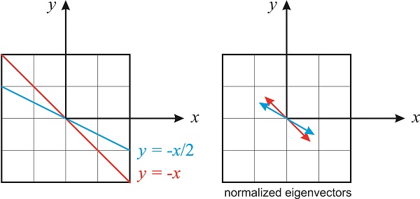
Figure \(\PageIndex{1}\) shows the lines \(y=-x\) and \(y=-x/2\). Any vector that lies along the line \(y=-x/2\) is an eigenvector with eigenvalue \(\lambda=2\), and any vector that lies along the line \(y=-x\) is an eigenvector with eigenvalue \(\lambda=1\). Eigenvectors that differ only in a constant factor are not treated as distinct. It is convenient and conventional to normalize the eigenvectors. Notice that we can calculate two normalized eigenvectors for each eigenvalue (pointing in one or the other direction), and the distinction between one or the other is not important.
In the first case, we have \(y=-x\). This means that any vector of the form \(\begin{pmatrix} a \\ -a \end{pmatrix}\) is an eigenvector, but we are looking for the value of \(a\) that makes this eigenvector normalized. In other words, we want \((a)^2+(-a)^2=1\), which gives \(a=\pm 1/\sqrt{2}\). In conclusion, both
\[\begin{array}{c c c} \dfrac{1}{\sqrt{2}}\begin{pmatrix} 1 \\ -1 \end{pmatrix} & \text{and} & \dfrac{1}{\sqrt{2}}\begin{pmatrix} -1 \\ 1 \end{pmatrix} \end{array} \nonumber \]
are normalized eigenvectors of
\[\mathbf{A}=\begin{pmatrix} 3&2 \\ -1&0 \end{pmatrix} \nonumber \]
with eigenvalue \(\lambda=1\).
For \(\lambda=2\), we have that \(y=-x/2\). This means that any vector of the form \(\begin{pmatrix} a \\ -a/2 \end{pmatrix}\) is an eigenvector, but we are looking for the value of \(a\) that makes this eigenvector normalized. In other words, we want \((a)^2+(-a/2)^2=1\), which gives \(a=\pm 2/\sqrt{5}\). In conclusion, both
\[\begin{array}{c c c} \dfrac{1}{\sqrt{5}}\begin{pmatrix} 2 \\ -1 \end{pmatrix} & \text{and} & \dfrac{1}{\sqrt{5}}\begin{pmatrix} -2 \\ 1 \end{pmatrix} \end{array} \nonumber \]
are normalized eigenvectors of
\[\mathbf{A}=\begin{pmatrix} 3&2 \\ -1&0 \end{pmatrix} \nonumber \]
with eigenvalue \(\lambda=2.\)
Find the eigenvalues and nomalized eigenvectors of
\[\mathbf{M}=\begin{pmatrix} 0&1 \\ -1&0 \end{pmatrix} \nonumber \]
The eigenvalues satisfy the characteristic equation:
\[\begin{vmatrix} -\lambda&1 \\ -1&-\lambda \end{vmatrix}=0\rightarrow (-\lambda)(-\lambda)-(1)(-1)=\lambda^2+1=0\rightarrow \lambda_{1,2}=\pm i \nonumber \]
For \(\lambda =i\):
\[\begin{pmatrix} 0&1 \\ -1&0 \end{pmatrix}\begin{pmatrix} x_1\\ y_1 \end{pmatrix}=i\begin{pmatrix} x_1\\ y_1 \end{pmatrix} \nonumber \]
\[y_1=ix_1 \nonumber \]
\[-x_1=i y_1 \nonumber \]
Again, the two equations we get have the same information (or more formally, are linearly dependent). From either one, we get \(y_1=i x_1\).
Any vector of the form
\[\mathbf{u}=\begin{pmatrix} a\\ ia \end{pmatrix} \nonumber \]
is an eigenvector of \(\mathbf{M}\) with eigenvalue \(\lambda=i\).
To normalize the vector (Section 14.4), we calculate the modulus of the vector using the dot product:
\[|\mathbf{u}|^2=\mathbf{u}^*\cdot\mathbf{u} \nonumber \]
(see Section 14.2 for a discussion of the dot product of complex vectors)
\[|\mathbf{u}|^2=\mathbf{u}^*\cdot\mathbf{u}=a^2+(ia)(-ia)=a^2+a^2=2a^2\rightarrow |\mathbf{u}|=\pm\sqrt{2}a \nonumber \]
and we divide the vector by its modulus.
The normalized eigenvectors for \(\lambda =i\) are, therefore,
\[\hat{\mathbf{u}}=\pm \dfrac{1}{\sqrt{2}}\begin{pmatrix} 1\\ i \end{pmatrix} \nonumber \]
For \(\lambda =-i\):
\[\begin{pmatrix} 0&1 \\ -1&0 \end{pmatrix}\begin{pmatrix} x_1\\ y_1 \end{pmatrix}=-i\begin{pmatrix} x_1\\ y_1 \end{pmatrix} \nonumber \]
\[y_1=-ix_1 \nonumber \]
\[-x_1=-i y_1 \nonumber \]
From either one, we get
\[y_1=-i x_1. \nonumber \]
Any vector of the form
\[\mathbf{v}=\begin{pmatrix} a\\ -ia \end{pmatrix} \nonumber \]
is an eigenvector of \(\mathbf{M}\) with eigenvalue \(\lambda=-i\).
To normalize the vector, we calculate the dot product:
\[|\mathbf{v}|^2=\mathbf{v}^*\cdot\mathbf{v}=a^2+(-ia)(ia)=a^2+a^2=2a^2\rightarrow |\mathbf{v}| =\pm\sqrt{2}a \nonumber \]
The normalized eigenvectors for \(\lambda =-i\) are, therefore,
\[\hat{\mathbf{v}}=\pm \dfrac{1}{\sqrt{2}}\begin{pmatrix} 1\\ -i \end{pmatrix} \nonumber \]
Matrix Eigenvalues: Some Important Properties
1)The eigenvalues of a triangular matrix are the diagonal elements.
\[\begin{pmatrix} a&b&c\\ 0&d&e\\ 0&0&f \end{pmatrix}\rightarrow \lambda_1=a;\;\lambda_2=d;\;\lambda_3=f \nonumber \]
2) If \(\lambda_1\),\(\lambda_2\)...,\(\lambda_n\), are the eigenvalues of the matrix \(\mathbf{A}\), then \(|\mathbf{A}|= \lambda_1\lambda_2...\lambda_n\)
3) The trace of the matrix \(\mathbf{A}\) is equal to the sum of all eigenvalues of the matrix \(\mathbf{A}\).
For example, for the matrix
\[\mathbf{A}=\begin{pmatrix} 1&1\\ -2&4 \end{pmatrix}\rightarrow |\mathbf{A}|=6=\lambda_1\lambda_2;\;Tr(\mathbf{A})=5=\lambda_1+\lambda_2 \nonumber \]
For a \(2\times 2\) matrix, the trace and the determinant are sufficient information to obtain the eigenvalues: \(\lambda_1=2\) and \(\lambda_2=3\).
4) Symmetric matrices-those that have a "mirror-plane" along the northeast-southwest diagonal (i.e. \(\mathbf{A}=\mathbf{A}^T\)) must have all real eigenvalues. Their eigenvectors are mutually orthogonal.
For example, for the matrix
\[\mathbf{A}=\begin{pmatrix} -2&4&0\\ 4&1&-1\\ 0&-1&-3 \end{pmatrix} \nonumber \]
the three eigenvalues are \(\lambda_1=1+\sqrt{21}\), \(\lambda_2=1-\sqrt{21}\), \(\lambda_3=-2\), and the three eigenvectors:
\[ \begin{array}{c} \mathbf{u}_1=\begin{pmatrix} -5-\sqrt{21}\\ -4-\sqrt{21}\\ 1 \end{pmatrix}, & \mathbf{u}_2=\begin{pmatrix} -5+\sqrt{21}\\ -4+\sqrt{21}\\ 1 \end{pmatrix}, & \text{and} & \mathbf{u}_3=\begin{pmatrix} 1\\ -1\\ 1 \end{pmatrix} \end{array} \nonumber \]
You can prove the eigenvectors are mutually orthogonal by taking their dot products.